B · Probability Distributions

Appendices

Executed in: Python · Book: ADM Appendix B

Probability distributions describe uncertainty about a quantity. This appendix lists the families used on this site, with their formulas, what their parameters do, and where they appear. It follows ADM Appendix B, adding the two discrete distributions used most often. Plots use this site’s own parameter choices.

At a glance

Table 1: The distributions used on this site (\(\Gamma\) is the gamma function; \(\alpha_0 = \sum_i \alpha_i\)).

Distribution	Parameters	Density or mass function	Mean	Variance
Bernoulli\((p)\)	\(p \in [0, 1]\)	\(P(x = 1) = p\), \(P(x = 0) = 1 - p\)	\(p\)	\(p(1 - p)\)
Categorical\((\mathbf{p})\)	\(p_i \ge 0\), \(\sum_i p_i = 1\)	\(P(x = i) = p_i\)	—	—
Uniform \(\mathcal{U}(a, b)\)	\(a < b\)	\(\frac{1}{b - a}\) on \([a, b]\)	\(\frac{a + b}{2}\)	\(\frac{(b - a)^2}{12}\)
Gaussian \(\mathcal{N}(\mu, \sigma^2)\)	\(\mu\), \(\sigma > 0\)	\(\frac{1}{\sigma\sqrt{2\pi}} e^{-(x - \mu)^2/(2\sigma^2)}\)	\(\mu\)	\(\sigma^2\)
Beta\((\alpha, \beta)\)	\(\alpha, \beta > 0\)	\(\frac{\Gamma(\alpha + \beta)}{\Gamma(\alpha)\Gamma(\beta)} x^{\alpha - 1}(1 - x)^{\beta - 1}\) on \((0, 1)\)	\(\frac{\alpha}{\alpha + \beta}\)	\(\frac{\alpha\beta}{(\alpha + \beta)^2(\alpha + \beta + 1)}\)
Gaussian \(\mathcal{N}(\boldsymbol{\mu}, \boldsymbol{\Sigma})\)	mean vector, covariance	see Equation 3	\(\boldsymbol{\mu}\)	\(\boldsymbol{\Sigma}\)
Dirichlet\((\boldsymbol{\alpha})\)	\(\alpha_i > 0\)	see Equation 4	\(\alpha_i / \alpha_0\)	\(\frac{\alpha_i(\alpha_0 - \alpha_i)}{\alpha_0^2(\alpha_0 + 1)}\)

Discrete distributions

A Bernoulli variable is a single yes/no outcome, like a coin toss or whether a click happens (the bandits of Chapter 15). A categorical variable takes one of \(n\) values with given probabilities: every discrete variable in a Bayesian network (Chapter 2), every row of a transition model \(T(s' \mid s, a)\), and every stochastic policy is one.

Uniform

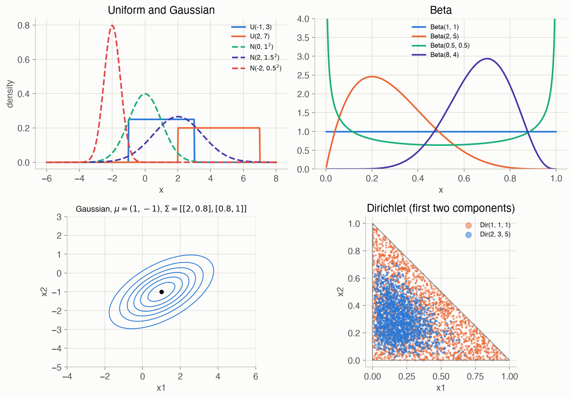
\(\mathcal{U}(a, b)\) spreads probability evenly over an interval: every point in \([a, b]\) is equally likely. It is the natural “know nothing but the range” distribution, used for random initial conditions and, as \(\text{Beta}(1, 1)\), as the uninformative prior of Chapter 4.

Gaussian

\[ \mathcal{N}(x \mid \mu, \sigma^2) = \frac{1}{\sigma\sqrt{2\pi}} \exp\!\Big(-\frac{(x - \mu)^2}{2\sigma^2}\Big) \tag{1}\]

In words. A bell curve centered at \(\mu\), whose width is set by \(\sigma\).

Term by term.

• \(\mu\): the mean, center and peak of the curve.
• \(\sigma\): the standard deviation; about 68% of the probability lies within \(\mu \pm \sigma\) and 95% within \(\mu \pm 1.96\sigma\).
• \(\frac{1}{\sigma\sqrt{2\pi}}\): the constant that makes the area 1.

Why it holds. \(\int e^{-z^2/2}\,dz = \sqrt{2\pi}\) (square the integral and switch to polar coordinates), and substituting \(z = (x - \mu)/\sigma\) gives the constant. The central limit theorem explains why the Gaussian is everywhere: sums of many small independent effects are approximately Gaussian. Used for continuous Bayesian networks (Chapter 2), exploration noise (Chapter 10–12) and Kalman filters (Chapter 19).

Beta

The Beta distribution describes an unknown probability, a number in \((0, 1)\). Its main use is as the conjugate prior for a Bernoulli probability:

\[ p \sim \text{Beta}(\alpha, \beta),\ \ \text{observe } k \text{ successes in } n \text{ trials} \quad\Longrightarrow\quad p \mid \text{data} \sim \text{Beta}(\alpha + k,\ \beta + n - k) \tag{2}\]

In words. Start with pseudo-counts \(\alpha\) and \(\beta\); add the observed successes and failures.

Term by term.

• \(\text{Beta}(1, 1)\) is uniform: no prior preference.
• The posterior mean \((\alpha + k)/(\alpha + \beta + n)\) moves from the prior mean toward the observed fraction \(k/n\) as \(n\) grows.
• Example: from a uniform prior, 7 successes in 10 trials give \(\text{Beta}(8, 4)\): mean 0.667, 95% interval 0.390 to 0.891.

Why it holds. By Bayes’ rule, the posterior is proportional to prior times likelihood: \(p^{\alpha - 1}(1 - p)^{\beta - 1} \cdot p^k(1 - p)^{n - k}\), which is the Beta form with exponents increased by \(k\) and \(n - k\). Used for parameter learning (Chapter 4), Bayesian bandits (Chapter 15) and failure-probability intervals (Chapter 14).

Multivariate Gaussian

\[ \mathcal{N}(\mathbf{x} \mid \boldsymbol{\mu}, \boldsymbol{\Sigma}) = \frac{1}{(2\pi)^{n/2} |\boldsymbol{\Sigma}|^{1/2}} \exp\!\Big(-\tfrac{1}{2}(\mathbf{x} - \boldsymbol{\mu})^\top \boldsymbol{\Sigma}^{-1}(\mathbf{x} - \boldsymbol{\mu})\Big) \tag{3}\]

In words. A bell-shaped hill in \(n\) dimensions, centered at \(\boldsymbol{\mu}\), stretched and tilted by \(\boldsymbol{\Sigma}\).

Term by term.

• \(\boldsymbol{\mu}\): the mean vector. \(\boldsymbol{\Sigma}\): the covariance matrix, symmetric and positive definite (Appendix A); its off-diagonal entries tilt the hill when variables are correlated.
• \((\mathbf{x} - \boldsymbol{\mu})^\top \boldsymbol{\Sigma}^{-1}(\mathbf{x} - \boldsymbol{\mu})\): the squared Mahalanobis distance; its level sets are the elliptical contours.
• \(|\boldsymbol{\Sigma}|\): the determinant, which normalizes for the ellipses’ volume.

Why it holds. Changing variables to \(\mathbf{z} = \mathbf{L}^{-1}(\mathbf{x} - \boldsymbol{\mu})\), with \(\boldsymbol{\Sigma} = \mathbf{L}\mathbf{L}^\top\), turns it into a product of \(n\) standard Gaussians; the Jacobian contributes \(|\boldsymbol{\Sigma}|^{1/2}\). Numerically, the example in Figure 1 integrates to 1.0000. Used for commute times (Chapter 3), the cross-entropy method (Chapter 10) and Kalman filters (Chapter 19).

Dirichlet

The Dirichlet generalizes the Beta to a whole probability vector, and is the conjugate prior for categorical variables:

\[ \text{Dir}(\mathbf{x} \mid \boldsymbol{\alpha}) = \frac{\Gamma(\alpha_0)}{\prod_{i=1}^{n} \Gamma(\alpha_i)} \prod_{i=1}^{n} x_i^{\alpha_i - 1}, \qquad x_i > 0,\ \sum_i x_i = 1,\ \ \alpha_0 = \sum_i \alpha_i \tag{4}\]

In words. A distribution over probability vectors: the \(\alpha_i\) act as pseudo-counts for each category.

Term by term.

• With all \(\alpha_i = 1\), every probability vector is equally likely.
• Larger \(\alpha_0\) concentrates the vectors near the mean \(\boldsymbol{\alpha}/\alpha_0\).
• Updating on counts \(m_i\) gives \(\text{Dir}(\boldsymbol{\alpha} + \mathbf{m})\), exactly as for the Beta.
• Example: \(\boldsymbol{\alpha} = (2, 3, 5)\) has mean \((0.2, 0.3, 0.5)\); 100,000 samples averaged 0.200, 0.300, 0.500.

Why it holds. The normalizing constant is the multivariate Beta function; with \(n = 2\) it reduces to the Beta distribution. Used for learning conditional probability tables (Chapter 4), Bayesian structure scores (Chapter 5) and posterior sampling of transition models (Chapter 16).

Checks

Table 2: Numerical checks of three densities.

Distribution	Area under density	Mean	Mean of 100,000 samples
Uniform(−1, 3)	1.000000	1.000	0.998
N(2, 1.5²)	1.000000	2.000	2.004
Beta(2, 5)	1.000000	0.286	0.287

Figures

Figure 1: Densities of the continuous families with this site’s example parameters. Top: uniform and Gaussian; Beta for several (α, β). Bottom: contours of a correlated two-dimensional Gaussian; 2,000 samples from Dirichlet(2, 3, 5) and Dirichlet(1, 1, 1), shown by their first two components.

Code

Python

import numpy as np
from scipy import stats

rng = np.random.default_rng(0)
posterior = stats.beta(1 + 7, 1 + 3)        # uniform prior, 7 of 10 successes
print("posterior mean", round(posterior.mean(), 3),
      "95% interval", np.round(posterior.ppf([0.025, 0.975]), 3))
samples = rng.dirichlet([2, 3, 5], 100_000)
print("Dirichlet sample mean", samples.mean(axis=0).round(3))
assert abs(posterior.mean() - 8 / 12) < 1e-12
assert np.allclose(samples.mean(axis=0), [0.2, 0.3, 0.5], atol=0.005)

Julia

import Distributions
using Random, Statistics

posterior = Distributions.Beta(1 + 7, 1 + 3)   # uniform prior, 7 of 10 successes
println("posterior mean ", round(Distributions.mean(posterior); digits = 3),
        ", 95% interval ", round.(Distributions.quantile.(posterior, [0.025, 0.975]); digits = 3))
x = rand(MersenneTwister(0), Distributions.Dirichlet([2.0, 3.0, 5.0]), 100_000)   # 3 × n
println("Dirichlet sample mean ", round.(vec(mean(x; dims = 2)); digits = 3))
@assert Distributions.mean(posterior) ≈ 8 / 12
@assert all(abs.(vec(mean(x; dims = 2)) .- [0.2, 0.3, 0.5]) .< 0.005)