14 · Policy Validation
Part II — Sequential Problems
Big picture
Where this chapter fits
Chapters 7–13 built ways to find good policies. Every one of them optimized a model: a transition function, a reward, a start distribution. Before a policy flies an aircraft or trades money, we need evidence that it does what we want in the world, not just in the model. Policy validation asks how well a policy performs on the metrics we care about, how sure we are of that answer, and how the answer changes when the model is wrong. This chapter closes Part II. Part III (Chapter 15 on) drops the assumption that the model is known at all.
The question: how do we measure a policy’s safety and performance, especially for rare failures, and how do we find the situations in which it breaks?
The short answer: evaluate the metrics exactly when the problem is small, and by simulation when it isn’t, always with error bars. Rare failures need importance sampling, which simulates dangerous situations more often and then corrects for it. Robustness analysis re-evaluates the policy on models that differ from the one it was optimized for. Trade analysis maps the compromises between metrics, such as safety and nuisance alerts. Adversarial analysis searches for the most likely way the policy fails.
The key ideas at a glance
A metric is an expectation over trajectories. Collision probability, expected advisory changes, and expected return are all averages of a per-trajectory score over the trajectories a policy produces. If the score adds up step by step, policy evaluation (Chapter 7) computes it exactly. Otherwise, or when the state space is too large, we simulate and average.
Every estimate needs an error bar. The standard error \(\hat\sigma / \sqrt{n}\) says how far the average of \(n\) simulations typically is from the truth. For a rare event, the relative standard error matters: an estimate of \(10^{-4}\) that is off by \(10^{-4}\) is useless, however small that error looks.
Importance sampling for rare events. Draw trajectories from a proposal that makes failures common, and weight each by how much more likely it was under the proposal than under the real model. The weighted average is still unbiased. The ideal proposal samples trajectories in proportion to how much they contribute. A proposal that pushes too hard produces a few enormous weights and can be worse than no proposal at all.
Robustness. A policy is only as good as its model. Re-evaluate it on plausible variations: noisier dynamics, a pilot who doesn’t always comply. Robust dynamic programming optimizes against the worst model in a set.
Trade analysis. Safety and efficiency compete. Varying a policy’s design parameters traces out the achievable pairs of metrics. Policies that are beaten on every metric by another policy are dominated; the rest form the Pareto front.
Adversarial analysis. Let an adversary choose the random outcomes, balancing “cause a failure” against “stay plausible”. The result is the most likely failure: a concrete story that engineers can inspect and judge.
Vocabulary
| Term | Plain meaning |
|---|---|
| Trajectory metric \(f_{\text{traj}}(\tau)\) | A score for one simulated trajectory, such as 1 if it ends in a collision |
| Performance metric \(f(\pi)\) | The expected trajectory metric under policy \(\pi\) |
| Standard error (SE) | Typical distance between a sample average and the true mean |
| Relative standard error | Standard error divided by the estimate; what matters for rare events |
| Proposal distribution \(P'(\tau)\) | The distribution we actually sample from in importance sampling |
| Importance weight \(w\) | \(P(\tau)/P'(\tau)\): corrects for sampling from the proposal |
| Effective sample size | How many unweighted samples the weighted ones are worth |
| Robust dynamic programming | Choose actions against the worst model in a set |
| Pareto front | The policies that no other policy beats on every metric |
| Most likely failure | The highest-probability trajectory that ends in failure |
After this chapter you can
- Evaluate a policy’s metrics exactly by policy evaluation, or by simulation with standard errors and confidence intervals.
- Estimate a rare-event probability with importance sampling, and recognize a proposal that makes things worse.
- Stress-test a policy on models it wasn’t designed for, and use robust dynamic programming.
- Build a trade-off curve and identify the Pareto front.
- Turn a policy into an adversarial search problem and find its most likely failure.
Intuition
TipAnalogy
A bridge has been designed on a computer. Before opening it, engineers:
- Measure its performance under typical traffic, and report the figure with a margin of error.
- Look for rare failures by loading the model with heavy trucks far more often than real traffic would, then scaling the results back down.
- Check robustness: what if the steel is 10% weaker than specified?
- Weigh trade-offs: a stiffer bridge is safer but costs more; which designs are not beaten on both counts?
- Play the adversary: what is the most plausible combination of wind, load and fatigue that brings it down?
Each check can send the design back to the drawing board.
Our running example is aircraft collision avoidance (ADM Appendix F.6, in the problem gallery). Our aircraft flies head on toward an intruder, which it would meet in 40 seconds. The state is our altitude \(h\) relative to the intruder, our vertical rate \(\dot h\), the previous advisory, and the time left \(t_{\text{col}}\). Every second the policy issues an advisory: none, descend at 5 m/s, or climb at 5 m/s. The pilot changes the vertical rate by at most 1 m/s per second, and random gusts add \(\pm 2\) m/s with probability ¼ each. A collision means passing within 50 m vertically. Each change of advisory costs 0.01, a collision costs 1. We compare two policies:
- the optimal policy for those costs, found by backward induction (Chapter 7);
- a simple policy: when the intruder is within 50 m vertically and less than 30 s away, climb if we are above it and descend if below.
Because the starting \(h\) and \(\dot h\) are whole numbers here, and every change is a whole number, the state stays on an integer grid. That makes exact evaluation possible, so every estimate on this page can be checked against the true answer.
Scoring a policy
From starts spread uniformly over \(\pm 200\) m and \(\pm 10\) m/s, the optimal policy collides with probability 6.42e-04 and changes its advisory 0.34 times per encounter on average. The simple policy collides with probability 0.072 and changes advisories 0.98 times. Both numbers are exact: they come from policy evaluation, the same backward sweep that computes a value function, but scoring collisions and changes instead of rewards. See Equation 1 and Equation 2.
How sure are we?
Simulating 10,000 encounters of the optimal policy gave 5 collisions: an estimate of 5.0e-04 with standard error 2.2e-04. That’s a relative error of 45%. To bring it down to 10%, direct simulation needs about 155,759 encounters. Meanwhile the average number of advisory changes, a common event, is already pinned down to 1.4% after 10,000. See Equation 3.
Make failures common, then correct
Instead of waiting for gusts to cause a collision, sample gusts that are more likely to cause one, and weight each simulated encounter by how much less likely it was in reality. A crude version, “push toward the intruder a bit more often”, cuts the error only a little: its relative error is 27% against 36% for direct sampling. Pushing much harder makes it worse (92%). A proposal guided by an estimate of the risk from each state does far better: 4.5% with the risk computed from a deliberately wrong model (Figure 6). See Equation 4 and Equation 5.
What if the model is wrong?
The optimal policy assumed the pilot always follows the advisory. If the pilot complies only 80% of the time, its collision probability rises to 3.8e-03, about 6 times higher. A policy optimized against the worse of the two models (always complies, or complies 80% of the time) keeps it at 1.4e-03, at the price of more advisory changes (Figure 7). See Equation 6.
Safety costs alerts
Lowering the cost of an advisory change makes the optimal policy more cautious: safer, but more disruptive. Plotting collision probability against advisory changes for many policies shows the achievable compromises. Of the 96 simple threshold policies we tried, 100% are beaten by some optimal policy on both metrics at once (Figure 8). See Equation 7.
How does it fail?
An adversary that controls the gusts can always cause a collision. The question is how unlikely its gusts must be. For the optimal policy, every start needs at least 3 gusts, each half as likely as calm air. For the simple policy, 2.0% of starts end in a collision with no gust at all (Figure 9). See Equation 8.
Formalism
Performance metrics
A trajectory \(\tau = (s_1, a_1, s_2, \ldots)\) produced by policy \(\pi\) from a start distribution \(b\) gets a score \(f_{\text{traj}}(\tau)\). The policy’s performance metric is its expectation (ADM §14.1):
\[ f(\pi) = \mathbb{E}_\tau\big[f_{\text{traj}}(\tau)\big], \qquad P(\tau) = b(s_1) \prod_t T\big(s_{t+1} \mid s_t, \pi(s_t)\big) \tag{1}\]
In words. Average the score over all the trajectories the policy can produce, each weighted by its probability.
Term by term.
- \(b(s_1)\) is the probability of the start state.
- Each factor \(T(s_{t+1} \mid s_t, \pi(s_t))\) is the probability of one transition when following the policy.
- With \(f_{\text{traj}} = 1\) for a collision and 0 otherwise, \(f(\pi)\) is the collision probability.
The expectation is only one summary. Tail measures, such as the 5th percentile of the return or the mean of the worst 5%, can matter more for safety.
When the score adds up over steps, the expectation is a value function:
\[ f_{\text{traj}}(\tau) = \sum_t f_{\text{step}}(s_t, a_t), \qquad f(\pi) = \sum_s f_{\text{state}}(s)\, b(s) \tag{2}\]
In words. If the score is a sum of per-step scores, treat the per-step score as a reward. Policy evaluation then gives its expected total from every state, \(f_{\text{state}}\). Average that over the start distribution.
Term by term. Advisory changes are additive: \(f_{\text{step}} = 1\) when \(a_t \ne a_{t-1}\). Collision is additive too, with a single nonzero term at \(t_{\text{col}} = 0\). In the code, evaluate runs this backward sweep for any per-step and final score.
Why it holds. Linearity of expectation: the expected sum is the sum of expected per-step scores. That is exactly the quantity a value function computes when the reward is \(f_{\text{step}}\) (Chapter 7, with \(\gamma = 1\) over a finite horizon).
Error bars for simulation
With \(n\) simulated trajectory scores \(x_1, \ldots, x_n\), sample mean \(\hat\mu\) and sample standard deviation \(\hat\sigma\):
\[ \text{SE} = \frac{\hat\sigma}{\sqrt n}, \qquad \text{relative SE} = \frac{\hat\sigma}{\hat\mu\sqrt n}, \qquad \text{95\% interval: } \hat\mu \pm 1.96\,\text{SE} \tag{3}\]
In words. The average of \(n\) samples wanders around the true mean by about \(\hat\sigma/\sqrt n\). Quadrupling the sample size halves the error.
Term by term.
- \(\hat\sigma\) is the spread of individual trajectory scores. For a 0/1 event with probability \(p\), it is \(\sqrt{p(1-p)}\).
- For that event, the relative SE is \(\sqrt{(1-p)/(np)} \approx 1/\sqrt{np}\): one over the square root of the number of failures observed. Ten failures give about 32% relative error, a hundred about 10%.
- The normal interval can extend below 0 for a rare event. The Bayesian alternative from Chapter 4, a \(\text{Beta}(1 + k, 1 + n - k)\) posterior after \(k\) failures in \(n\) trials, never does.
Why it holds. The variance of a sum of \(n\) independent samples is \(n\sigma^2\), so the variance of their average is \(\sigma^2/n\). The central limit theorem makes the average approximately normal, which gives the 1.96.
Importance sampling
To estimate \(f(\pi)\) from trajectories drawn from a proposal \(P'\) instead of \(P\) (ADM §14.2):
\[ f(\pi) = \sum_\tau f_{\text{traj}}(\tau)\, P(\tau) = \sum_\tau f_{\text{traj}}(\tau)\, \frac{P(\tau)}{P'(\tau)}\, P'(\tau) \approx \frac1n \sum_{i=1}^n f_{\text{traj}}(\tau^{(i)})\, \frac{P(\tau^{(i)})}{P'(\tau^{(i)})}, \quad \tau^{(i)} \sim P' \tag{4}\]
In words. Sample from a distribution that produces the interesting trajectories more often, and down-weight each one by how much more often it was produced than it should have been.
Term by term.
- \(w^{(i)} = P(\tau^{(i)})/P'(\tau^{(i)})\) is the importance weight. A failure that the proposal makes 100 times more likely counts \(1/100\).
- \(P'\) must give positive probability to every trajectory that \(P\) does and that has \(f_{\text{traj}} \neq 0\). Otherwise those trajectories are never seen, and the estimate is biased.
- With \(P(\tau)\) from Equation 1, the start and policy terms cancel if the proposal only changes the noise. The weight is then a product of per-step ratios \(P(\nu_t)/P'(\nu_t)\). That’s what
simulateaccumulates, in logs.
Why it holds. Multiplying and dividing by \(P'(\tau)\) changes nothing. The second sum is an expectation under \(P'\), and a sample average estimates it without bias. This is the same idea as likelihood weighting in Bayesian networks (Chapter 3).
Which proposal is best?
\[ P^*(\tau) = \frac{|f_{\text{traj}}(\tau)|\, P(\tau)}{\sum_{\tau'} |f_{\text{traj}}(\tau')|\, P(\tau')}, \qquad P'(\nu \mid s) \propto P(\nu)\, \hat U\big(s'(s, \nu)\big) \tag{5}\]
In words. The ideal proposal samples each trajectory in proportion to its contribution to the answer. For a sequential problem, that can be done one step at a time: choose each random outcome in proportion to its probability times the risk that remains afterward.
Term by term.
- For a nonnegative \(f_{\text{traj}}\) the denominator of \(P^*\) is \(f(\pi)\) itself, the unknown. So \(P^*\) is a target to approximate, not something we can use directly.
- On the right, \(\hat U(s')\) is an estimate of the risk-to-go: the probability of a failure from the next state \(s'\) onward. With the exact risk-to-go this reproduces \(P^*\) and every weighted sample equals the start state’s risk, so the estimate’s only noise is from the start states. With an approximate \(\hat U\) (here, computed from a model with larger gusts), it is still very good.
- We add a small constant to \(\hat U\) so that no outcome gets probability 0 (the support condition above).
Why it holds. Under \(P^*\) with \(f_{\text{traj}} \ge 0\), every sample’s weighted value is \(f_{\text{traj}}(\tau)P(\tau)/P^*(\tau) = f(\pi)\): zero variance. For the step-by-step form, write the risk-to-go as \(U(s) = \sum_\nu P(\nu)\, U(s'(s, \nu))\). Choosing \(\nu\) with probability \(P(\nu)U(s')/U(s)\) gives a step weight of \(U(s)/U(s')\). Along a failing trajectory these ratios telescope to \(U(s_1)/U(s_{\text{end}}) = U(s_1)\), because the final risk of a failure is 1.
Robustness and robust dynamic programming
Evaluate the policy on models other than the one it was optimized for: stress testing (ADM §14.3). If it is too sensitive, optimize against a set of models \((T_1, R_1), \ldots, (T_n, R_n)\) at once (G. N. Iyengar, Mathematics of Operations Research, 2005):
\[ U_{k+1}(s) = \max_a\ \min_i\ \Big(R_i(s, a) + \gamma \sum_{s'} T_i(s' \mid s, a)\, U_k(s')\Big) \tag{6}\]
In words. Score each action by the model that is worst for it, then pick the action with the best worst case.
Term by term.
- The \(\min_i\) is taken separately for each state and action: the “worst model” can differ from place to place.
- With a single model, this is the ordinary Bellman update (Chapter 7).
- In the code we minimize cost rather than maximize reward, so the update reads \(\min_a \max_i\).
Why it holds. It is the Bellman update of a game in which nature picks the model after seeing our action. The result guarantees at least \(U(s)\) against any sequence of models chosen from the set.
Trade analysis
For several metrics \(f_1, \ldots, f_k\), all to be minimized (ADM §14.4):
\[ \pi' \text{ dominates } \pi \iff f_j(\pi') \le f_j(\pi) \text{ for all } j \text{ and } f_j(\pi') < f_j(\pi) \text{ for some } j \tag{7}\]
In words. One policy dominates another if it is at least as good on every metric and strictly better on one. The Pareto front is the set of policies nothing dominates.
Term by term. Metrics to be maximized are negated first. Dominated policies can be discarded whatever the relative importance of the metrics. Choosing among the policies on the front is a value judgment, such as how many nuisance alerts one avoided collision is worth.
A single weighted objective \(\theta f_1 + (1 - \theta) f_2\), optimized for each \(\theta\), traces part of the front. That is what varying the cost of an advisory change does in Figure 8.
Adversarial analysis
Turn validation into search (ADM §14.5). An adversary picks the next state as its action, among those our policy can lead to. Its reward is
\[ R'(s, s') = -R\big(s, \pi(s)\big) + \lambda \log T\big(s' \mid s, \pi(s)\big) \tag{8}\]
In words. The adversary wants us to do badly, but pays for every unlikely outcome it chooses. \(\lambda\) sets the exchange rate between our loss and plausibility.
Term by term.
- \(-R\) is our cost, so the adversary gains when we lose.
- \(\log T\) is the log-probability of the outcome it chose. Summed over the trajectory, it is the trajectory’s log-likelihood.
- Small \(\lambda\): the adversary causes a failure whatever it takes. Large \(\lambda\): it follows the most likely trajectory, failure or not.
- The adversarial transitions are deterministic (the next state is the adversary’s action), so this is a search problem that dynamic programming solves exactly on our lattice.
- This \(\lambda\) is unrelated to GAE’s \(\lambda\) in Chapter 13.
To find the most likely failure, keep only the log-probabilities as rewards and require the trajectory to end in a failure: a terminal reward of 0 for a failure and \(-\infty\) otherwise (eq. 14.16 in the book). The answer is the highest-probability trajectory among those that fail.
Worked example
Error bars by hand
The first 10,000 simulated encounters of the optimal policy contained \(k =\) 5 collisions.
- Estimate: \(\hat\mu = k/n =\) 5.0e-04.
- Spread: \(\hat\sigma \approx \sqrt{\hat\mu(1 - \hat\mu)} =\) 0.0224.
- Standard error: \(\hat\sigma/\sqrt{10{,}000} =\) 2.2e-04, a relative error of 45%.
- 95% normal interval: (6.2e-05, 9.4e-04). The Beta posterior’s 95% interval is (2.2e-04, 1.2e-03).
The true value, from exact evaluation, is 6.42e-04. Both intervals contain it, but both are wide: the upper end is 15 times the lower end for the normal interval and 5.3 times for the Beta interval.
One importance weight
Take a state below the intruder (\(h < 0\)), where an upward push of +2 m/s is “toward” it. The tilt proposal with strength 1 multiplies each outcome’s probability by \(e^{+1}\) (toward), \(e^0\) (calm) or \(e^{-1}\) (away), then renormalizes:
| Outcome | \(P(\nu)\) | \(P'(\nu)\) | Ratio \(P/P'\) |
|---|---|---|---|
| away, −2 | 0.25 | 0.072 | 3.46 |
| calm, 0 | 0.50 | 0.393 | 1.27 |
| toward, +2 | 0.25 | 0.534 | 0.47 |
Three steps with outcomes toward, calm, toward get weight 0.47 × 1.27 × 0.47 = 0.278. Over 40 steps these factors multiply. A trajectory with many “away” steps gets a weight of 3.5 per step, so a handful of such trajectories can carry enormous weight. That is why a strong tilt made the estimate worse.
Who dominates whom?
Four policies, scored exactly (collision probability, advisory changes):
| Policy | Collision probability | Advisory changes | On the front? |
|---|---|---|---|
| simple, 50 m / 30 s | 7.25e-02 | 0.98 | no |
| simple, 150 m / 30 s | 2.43e-03 | 1.38 | no |
| simple, 200 m / 40 s | 2.08e-04 | 1.89 | yes |
| optimal, change cost 0.01 | 6.42e-04 | 0.34 | yes |
The optimal policy has both fewer collisions and fewer changes than the first two simple policies, so it dominates them. The 200 m / 40 s simple policy has fewer collisions than the optimal one, but it changes advisories much more often, so neither dominates the other. Among these four, the front is the optimal policy and that one simple policy.
Interactive
Explore the trade-off
Move the simple policy’s thresholds and see where it lands among all the policies of Figure 8. The blue curve is the optimal policy for different costs of an advisory change. A simple policy on or near that curve is as good as it gets for its number of alerts.
Play the adversary
Pick a start and the adversary’s \(\lambda\). The adversary controls every gust, trading “cause a collision” against “stay likely” (Equation 8). Dots mark its gusts; the shaded band is the collision zone at \(t_{\text{col}} = 0\). Small \(\lambda\) buys a collision with many gusts; at large \(\lambda\) it stops paying for gusts and the encounter ends safely.
Grey dots mean no advisory, orange descend, blue climb. A triangle pointing up is an upward gust (+2 m/s), pointing down a downward one.
Algorithms & code
Estimating a metric
def mc_estimate(x: Array, level: float = 0.95):
    """Mean of samples x with its standard error (eq. 14.5), relative
    standard error (eq. 14.6) and a normal confidence interval.
    Returns (mean, se, relative_se, (low, high))."""
    x = np.asarray(x, dtype=float)
    mean = x.mean()
    se = x.std(ddof=1) / np.sqrt(len(x))      # sample sd / sqrt(n)
    z = stats.norm.ppf(0.5 + level / 2)       # 1.96 for 95%
    rel = se / mean if mean != 0 else np.inf
    return mean, se, rel, (mean - z * se, mean + z * se)

def beta_interval(k: int, n: int, level: float = 0.95):
    """Bayesian interval for a probability after k successes in n trials,
    from the Beta(1 + k, 1 + n - k) posterior of a uniform prior (Ch 4).
    Unlike the normal interval, it never goes below 0."""
    post = stats.beta(1 + k, 1 + n - k)
    return post.ppf(0.5 - level / 2), post.ppf(0.5 + level / 2)

def evaluate(model, policy, step_metric=None, final_metric=None,
             history=False):
    """Exact policy evaluation of an additive metric (eq. 14.3) by
    backward induction.

    step_metric(a_prev, a) scores each step (default: 0) and
    final_metric is a (n_h, n_hdot) array scored at t_col = 0 (default:
    the collision indicator). Returns V[a_prev, i_h, i_hdot] at
    t_col = T_START: the expected total from each start state. With
    history=True, returns the list of V at t_col = 0, 1, ..., T_START.
    """
    final = collided(model) if final_metric is None else final_metric
    V = np.repeat(final[None], 3, axis=0)
    Vs = [V]
    a_prev = np.arange(3)[:, None, None]
    i = np.arange(V.shape[1])[:, None]            # row index, broadcasts
    j = np.arange(V.shape[2])[None, :]            # column index
    for t in range(1, T_START + 1):
        EV = expect(model, V)                     # (a, n_h, n_hdot)
        a = policy[t]                             # (a_prev, n_h, n_hdot)
        V = EV[a, i, j]                           # V[p, i, j] = EV[a[p, i, j], i, j]
        if step_metric is not None:
            V = V + step_metric(a_prev, a)
        Vs.append(V)
    return Vs if history else V
using ADM, Random, Statistics
import Distributions
# Mean, standard error (eq. 14.5), relative standard error (eq. 14.6), 95% interval.
function mc_estimate(x)
μ, se = mean(x), std(x) / sqrt(length(x)) # std uses n - 1, like ddof=1
return μ, se, se / μ, (μ - 1.96se, μ + 1.96se)
end
# Bayesian interval after k successes in n trials: Beta(1 + k, 1 + n - k) posterior.
beta_interval(k, n) = Distributions.quantile.(Distributions.Beta(1 + k, 1 + n - k), (0.025, 0.975))
m = CAModel()
policy, _ = ca_optimal_policy(m)
exact = ca_start_average(m, ca_evaluate(m, policy)) # exact, by policy evaluation
# Direct simulation from uniform integer starts.
rng = MersenneTwister(0)
# Float64 turns each true/false into 1.0/0.0 so mean and std are ordinary numbers.
hits = [Float64(abs(ca_simulate(m, policy, rand(rng, -CA_H_START:CA_H_START),
rand(rng, -CA_HDOT_START:CA_HDOT_START), rng)[1]) < CA_COLLISION_H)
for _ in 1:100_000]
μ, se, rel, ci = mc_estimate(hits)
println("exact $(round(exact; sigdigits = 3)), estimate $(round(μ; sigdigits = 3)) ± $(round(se; sigdigits = 2))")
@assert abs(μ - exact) < 4se
@assert beta_interval(sum(hits), length(hits))[1] > 0Importance sampling
def importance_estimate(f: Array, log_w: Array):
    """Importance sampling estimate of E_P[f] from samples drawn from a
    proposal P', with log_w = log P(tau) - log P'(tau) (eq. 14.12).

    Returns (mean, se, ess). The effective sample size
    ess = (sum w)^2 / sum w^2 says how many direct samples the weighted
    ones are worth for estimating the weights' spread; it collapses when
    a few huge weights dominate.
    """
    w = np.exp(np.asarray(log_w, dtype=float))
    fw = np.asarray(f, dtype=float) * w       # each sample's contribution
    n = len(fw)
    return fw.mean(), fw.std(ddof=1) / np.sqrt(n), w.sum()**2 / (w**2).sum()

def simulate(model, policy, h, hdot, rng, tilt=0.0, guide=None, eps=1e-6,
             record=False):
    """Roll out len(h) episodes side by side from integer starts h, hdot.

    By default the noise is drawn from the model. Two proposals bias it
    toward collisions, for importance sampling:
      tilt > 0: P'(nu) is proportional to P(nu) exp(tilt * s), where
        s = +1 for a push toward the intruder (it reduces |h|), -1 for a
        push away and 0 for nu = 0;
      guide: risk-to-go tables from evaluate(..., history=True). P'(nu)
        is proportional to P(nu) (guide[t-1](next state) + eps): eq. 14.13
        applied one step at a time. eps keeps every branch possible.
    The returned log weights, sum log P(nu) / P'(nu), undo the bias
    (eq. 14.12); without a proposal they are all 0.

    Returns (h_final, changes, log_w), plus the (n, T_START + 1) altitude
    paths when record is True. The dynamics are exact (no clamping); only
    the policy lookup clamps to the lattice.
    """
    h, hdot = np.array(h), np.array(hdot)
    n = len(h)
    a_prev = np.zeros(n, dtype=int)
    changes, log_w = np.zeros(n), np.zeros(n)
    path = [h.copy()]
    nus, p_nu = zip(*model.noise_outcomes())
    for t in range(T_START, 0, -1):
        a = policy[t][(a_prev,) + _index(model, h, hdot)]
        changes += a != a_prev
        comply = rng.random(n) < model.compliance
        acc = np.zeros(n, dtype=int)
        for k in (1, 2):                  # advised rates; "none" keeps 0
            m = comply & (a == k)
            acc[m] = accel(model, hdot[m], k)
        h2 = h + hdot                     # the next altitude uses the old rate
        # Proposal weight of each noise value, shape (3, n), unnormalized.
        w = np.array([np.full(n, p) for p in p_nu])
        if tilt:
            toward = -np.sign(h)          # +1 below the intruder, -1 above
            w *= np.exp(tilt * np.sign(nus)[:, None] * toward)
        if guide is not None:
            for k, nu in enumerate(nus):
                # guide[t - 1][a_prev', i_h', i_hdot'] with a_prev' = a.
                w[k] *= guide[t - 1][(a,) + _index(model, h2, hdot + acc + nu)] + eps
        q = w / w.sum(axis=0)             # proposal probabilities P'(nu)
        # Inverse-CDF draw of the branch: count the cumulative
        # probabilities below u (the min guards against rounding).
        k = np.minimum((rng.random(n) > np.cumsum(q, axis=0)).sum(axis=0), 2)
        log_w += np.log(np.take(p_nu, k)) - np.log(q[k, np.arange(n)])
        h, hdot, a_prev = h2, hdot + acc + np.take(nus, k), a
        path.append(h.copy())
    out = (h, changes, log_w)
    return out + (np.array(path).T,) if record else out
using ADM, Random, Statistics
m = CAModel()
policy, _ = ca_optimal_policy(m)
risk = ca_evaluate(m, policy; history = true) # risk[t + 1]: risk-to-go at t_col = t
exact = ca_start_average(m, risk[end])
# One guided encounter: choose each gust with probability ∝ P(ν) (risk after it + ε)
# (eq. 14.13 one step at a time) and return (collided?, log weight).
function guided_rollout(h, ḣ, rng; ε = 1e-6)
a_prev, logw = 1, 0.0
noise = ADM.ca_noise(m) # ((ν, P(ν)) for ν = -2, 0, 2)
for t in CA_T_START:-1:1
a = policy[t][a_prev, ca_index(m, h, ḣ)...]
acc = ADM.ca_accel(m, ḣ, a)
# Proposal weights: P(ν) times the risk-to-go of the state after ν.
w = [p * (risk[t][a, ca_index(m, h + ḣ, ḣ + acc + ν)...] + ε) for (ν, p) in noise]
q = w ./ sum(w)
k = min(searchsortedfirst(cumsum(q), rand(rng)), 3) # inverse-CDF draw
logw += log(noise[k][2]) - log(q[k]) # log P(ν) - log P'(ν)
h, ḣ, a_prev = h + ḣ, ḣ + acc + noise[k][1], a
end
return abs(h) < CA_COLLISION_H, logw
end
# Importance sampling estimate (eq. 14.12): mean of f × w, with its standard error.
function importance_estimate(f, logw)
fw = f .* exp.(logw)
return mean(fw), std(fw) / sqrt(length(fw))
end
rng = MersenneTwister(1)
runs = [guided_rollout(rand(rng, -200:200), rand(rng, -10:10), rng) for _ in 1:2_000]
μ, se = importance_estimate(first.(runs), last.(runs))
println("exact $(round(exact; sigdigits = 4)), guided estimate $(round(μ; sigdigits = 4)) ± $(round(se; sigdigits = 2))")
@assert abs(μ - exact) < 4se && se < 0.05exactRobustness and trade-offs
def optimal_policy(model=Model(), models=None):
    """Backward induction for the minimum expected cost.

    Returns (policy, cost): policy[t, a_prev, i_h, i_hdot] is the advisory
    at t_col = t (row 0 is unused) and cost[a_prev, i_h, i_hdot] is the
    optimal expected cost at t_col = T_START. With `models`, a list of
    Models, it is robust dynamic programming: each advisory is scored by
    its worst model, then the best advisory is chosen.
    """
    models = models or [model]
    change = model.change_cost * (1 - np.eye(3))  # change[a_prev, a]
    U = np.repeat(model.collision_cost * collided(model)[None], 3, axis=0)
    policy = np.zeros((T_START + 1,) + U.shape, dtype=np.int8)
    for t in range(1, T_START + 1):
        EU = np.max([expect(m, U) for m in models], axis=0)  # worst model
        # Q[a_prev, a, ...]: cost of switching to a, then continuing.
        Q = change[:, :, None, None] + EU[None]
        policy[t] = Q.argmin(axis=1)
        U = Q.min(axis=1)
    return policy, U

def pareto_front(points: Array) -> Array:
    """Boolean mask of the rows of points (n, k) that no other row
    dominates, where every metric is to be minimized. Row j dominates
    row i if it is no worse on every metric and better on at least one."""
    P = np.asarray(points, dtype=float)
    # no_worse[i, j]: row j is <= row i everywhere; better: < somewhere.
    no_worse = (P[None, :, :] <= P[:, None, :]).all(axis=2)
    better = (P[None, :, :] < P[:, None, :]).any(axis=2)
    return ~(no_worse & better).any(axis=1)
using ADM
# Rows of `points` that no other row dominates (all metrics minimized, eq. on Pareto dominance).
function pareto_front(points)
n = size(points, 1)
dominates(j, i) = all(points[j, :] .<= points[i, :]) && any(points[j, :] .< points[i, :])
return [!any(dominates(j, i) for j in 1:n if j != i) for i in 1:n]
end
m, worse = CAModel(), CAModel(compliance = 0.8)
nominal, _ = ca_optimal_policy(m)
robust, _ = ca_optimal_policy(m; models = [m, worse]) # robust dynamic programming (eq. 14.14)
collision(policy, model) = ca_start_average(model, ca_evaluate(model, policy))
advisory_changes(policy) = ca_start_average(m, ca_evaluate(m, policy; step_metric = (p, a) -> p != a,
final = zeros(1001, 61)))
for (name, p) in (("nominal", nominal), ("robust", robust))
println(name, ": collision ", round(collision(p, m); sigdigits = 3), " (complies), ",
round(collision(p, worse); sigdigits = 3), " (80%), changes ", round(advisory_changes(p); digits = 3))
end
@assert collision(robust, worse) < collision(nominal, worse)
# Simple threshold policies: altitude thresholds 50, 100, 150, 200 m, time 30 s.
pts = [[collision(ca_simple_policy(m; h_thresh = h), m), advisory_changes(ca_simple_policy(m; h_thresh = h))]
for h in (50, 100, 150, 200)]
println("on the Pareto front: ", pareto_front(permutedims(hcat(pts...))))Adversarial analysis
def adversary(model, policy, lam=None):
    """Solve the adversarial problem for a fixed policy (ADM §14.5).

    The adversary picks each transition's outcome (compliance and noise
    branch). Its step reward is our cost plus lam * log T(branch), and
    it also collects our collision cost at t_col = 0 (eq. 14.15). With
    lam=None it looks for the most likely failure instead (eq. 14.16):
    step reward log T(branch), 0 for ending in a collision, -inf for not.

    Returns (W, choice): W[a_prev, i_h, i_hdot] is the adversary's best
    total from each state at t_col = T_START, and choice[t] (same shape)
    is the index of its best branch at t_col = t, in the order of
    outcomes(). Deterministic search, so dynamic programming is exact.
    """
    hit = collided(model)
    if lam is None:
        W = np.where(hit > 0, 0.0, -np.inf)
        W = np.repeat(W[None], 3, axis=0)
    else:
        W = np.repeat(model.collision_cost * hit[None], 3, axis=0)
    a_prev = np.arange(3)[:, None, None]
    i = np.arange(W.shape[1])[:, None]
    j = np.arange(W.shape[2])[None, :]
    choice = [None]
    for t in range(1, T_START + 1):
        # best[a, k]: value of branch k after advisory a, for every state.
        best = np.array([[(np.log(p) if lam is None else lam * np.log(p)) + W[a][ih, idd]
                          for ih, idd, p in outcomes(model, a)] for a in range(3)])
        a = policy[t]                                 # (a_prev, n_h, n_hdot)
        per_branch = best[a, :, i, j]                 # (a_prev, n_h, n_hdot, k)
        choice.append(per_branch.argmax(axis=-1))
        W = per_branch.max(axis=-1)
        if lam is not None:
            W = W + model.change_cost * (a != a_prev)
    return W, choice

def replay(model, policy, choice, h, hdot):
    """Follow the adversary's choices from one start (h, hdot).
    Returns a list of (t_col, h, hdot, advisory, nu) per step, then the
    final (0, h, hdot, None, None)."""
    a_prev, steps = 0, []
    for t in range(T_START, 0, -1):
        ih, idd = _index(model, h, hdot)
        a = int(policy[t][a_prev, ih, idd])
        k = int(choice[t][a_prev, ih, idd])
        # Recover the branch: compliance outer loop, noise inner loop.
        branches = [(c, nu) for c, pc in ((True, model.compliance),
                                          (False, 1 - model.compliance)) if pc > 0
                    for nu, _ in model.noise_outcomes()]
        comply, nu = branches[k]
        acc = int(accel(model, np.array(hdot), a)) if comply else 0
        steps.append((t, h, hdot, a, nu))
        h, hdot, a_prev = h + hdot, hdot + acc + nu, a
    steps.append((0, h, hdot, None, None))
    return steps
using ADM
m = CAModel()
policy, _ = ca_optimal_policy(m)
simple = ca_simple_policy(m)
# W[a_prev, i, j]: best log-probability of a path that ends in a collision (eq. 14.16).
# Each gust (probability ¼) is half as likely as calm air (½), so a path with k gusts
# has log-probability 40 log ½ - k log 2.
function gusts_needed(policy)
W = ca_most_likely_failure(m, policy)
Ws = W[1, (-200:200) .+ (m.h_max + 1), (-10:10) .+ (m.hdot_max + 1)] # starts; a_prev = none
return round.(Int, (CA_T_START * log(0.5) .- Ws) ./ log(2))
end
g_opt, g_simple = gusts_needed(policy), gusts_needed(simple)
println("optimal policy: at least $(minimum(g_opt)) gusts from any start")
println("simple policy: $(round(100 * sum(g_simple .== 0) / length(g_simple); digits = 1))% of starts fail in calm air")
@assert minimum(g_opt) >= 3 && any(g_simple .== 0)
NoteReading the Julia code (for Python programmers)
policy[t][a_prev, ca_index(m, h, ḣ)...]:...splats the tuple of two indices into the indexing call, likepolicy[t][(a_prev,) + idx]in Python.risk[t]is the risk at \(t_{\text{col}} = t - 1\): Julia arrays start at 1, so the list of values from \(t_{\text{col}} = 0\) to 40 is indexed 1 to 41.- Advisories are 1, 2, 3 (none, descend, climb) in Julia and 0, 1, 2 in Python.
first.(runs)appliesfirstto each tuple, like[r[0] for r in runs].import Distributionswith qualified names avoids clashes with other packages’ exports (§6.1 of the site’s conventions).
Run them
m = ca.Model()
policy, cost = ca.optimal_policy(m)
exact = ca.start_average(m, ca.evaluate(m, policy))

rng = np.random.default_rng(7)
starts = ca.sample_starts(10_000, rng)
h_end, _, _ = ca.simulate(m, policy, *starts, rng)
direct = mc_estimate(np.abs(h_end) < ca.COLLISION_H)

risk = ca.evaluate(ca.Model(noise=3), policy, history=True)   # a rough model's risk-to-go
h_end, _, log_w = ca.simulate(m, policy, *starts, rng, guide=risk)
guided = importance_estimate(np.abs(h_end) < ca.COLLISION_H, log_w)
exact 6.416e-04; direct 4.00e-04 ± 2.0e-04; guided 6.349e-04 ± 2.6e-05 (effective sample size 29)Results
The two policies and their risk
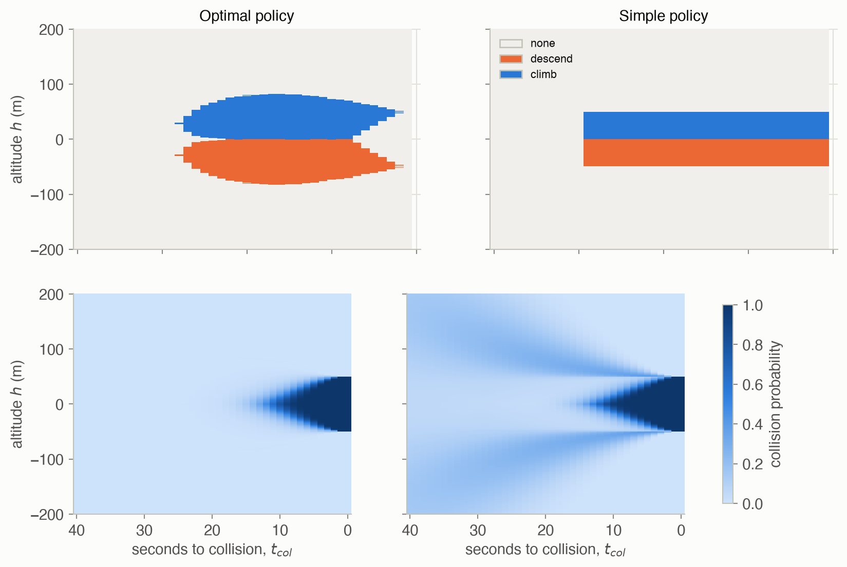
- The optimal policy waits. At rate 0 it issues no advisory until about 25 s before the encounter. Each advisory has a cost, and far out, the gusts will often carry the aircraft clear anyway. Its advisory region is widest, about ±80 m, around 10 s out. It narrows in the last seconds, where an advisory can no longer change the outcome.
- The simple policy reacts only inside its fixed ±50 m band. Its risk map has two ridges of moderate risk well away from the intruder. From those states, gusts tend to carry the aircraft to the edge of the band late in the encounter, and the policy acts only once inside it.
- Close in and late, even the optimal policy collides. The pilot can change the rate by only 1 m/s each second.
Direct simulation converges slowly for rare events
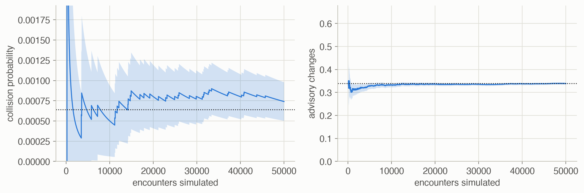
After all 50,000 encounters, the collision estimate rests on 37 collisions. Each one makes the estimate jump, and it decays between them. The advisory-change estimate converges within a few thousand encounters, because changes are common: 0.34 per encounter on average.
Importance sampling: the proposal is everything
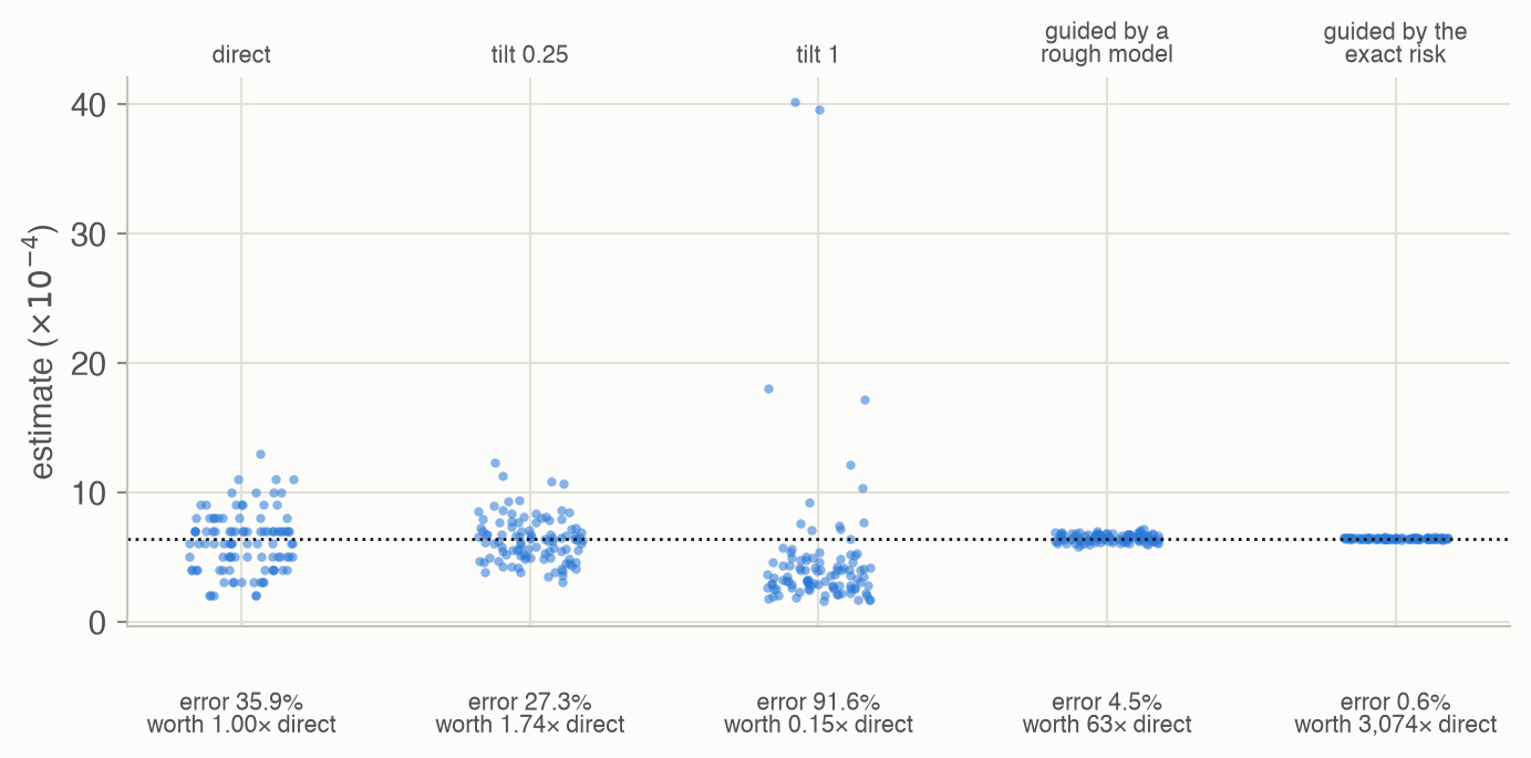
- Direct sampling sees about 6 collisions per run, so each estimate is a small whole number divided by 10,000.
- Tilting the gusts toward the intruder helps a little at strength 0.25 (51 collisions per run). At strength 1 there are 1,667 collisions per run, but their weights vary wildly: the effective sample size averages only 10 of 10,000. Most estimates fall below the truth and a few far above it. That is the signature of heavy-tailed weights: unbiased on average, useless in any single run.
- Guided proposals follow Equation 5. With the exact risk-to-go, the error is 0.6%, but computing that risk already answers the question. The practical case uses a risk estimate from a cheaper or cruder model. Here it came from a model with ±3 m/s gusts instead of ±2, and the error was still 4.5%: as good as about 63 times as many direct samples.
Robustness to the pilot
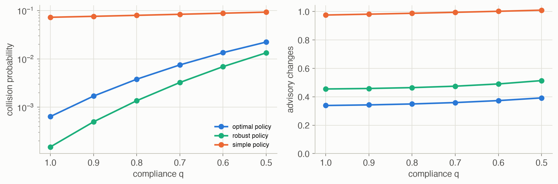
- The optimal policy is sensitive to compliance. Its collision probability rises from 6.4e-04 with full compliance to 3.8e-03 at 80% and 2.2e-02 at 50%. Stronger gusts hurt it too: ±3 m/s gives 8.6e-03 and ±4 m/s gives 2.1e-02.
- The robust policy is safer under every compliance level shown, including full compliance, where its collision probability is 1.5e-04. It pays with more advisory changes: 0.46 against 0.34.
- Part of that gain is simply more caution. An ordinary optimal policy with a lower change cost (0.002) alerts about as often, 0.44 changes, and has collision probability 1.6e-03 at 80% compliance, against the robust policy’s 1.4e-03. So robust dynamic programming buys caution where it helps most, and a little extra safety on top.
Trade-offs
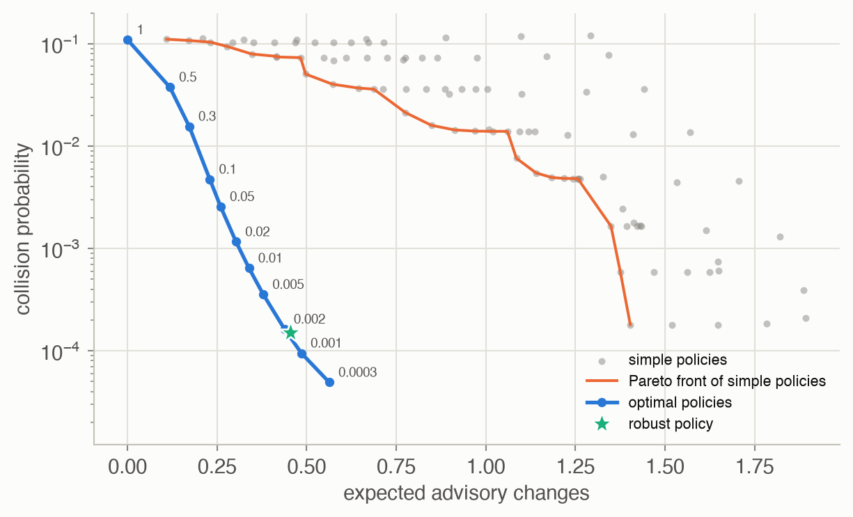
27 of the 96 simple policies are on their own Pareto front, but the optimal curve is better still: 100% of the simple policies are dominated by one of the 11 optimal policies shown. With a change cost of 1 or more, the optimal policy never alerts (collision probability 0.109): no advisory is worth its cost.
The robust policy sits just above the curve. Under the nominal model, its collision probability, 1.51e-04, is a little higher than the 1.34e-04 of an optimal policy with the same alert rate (interpolated along the curve). That is the price of its insurance against non-compliance.
The most likely failure
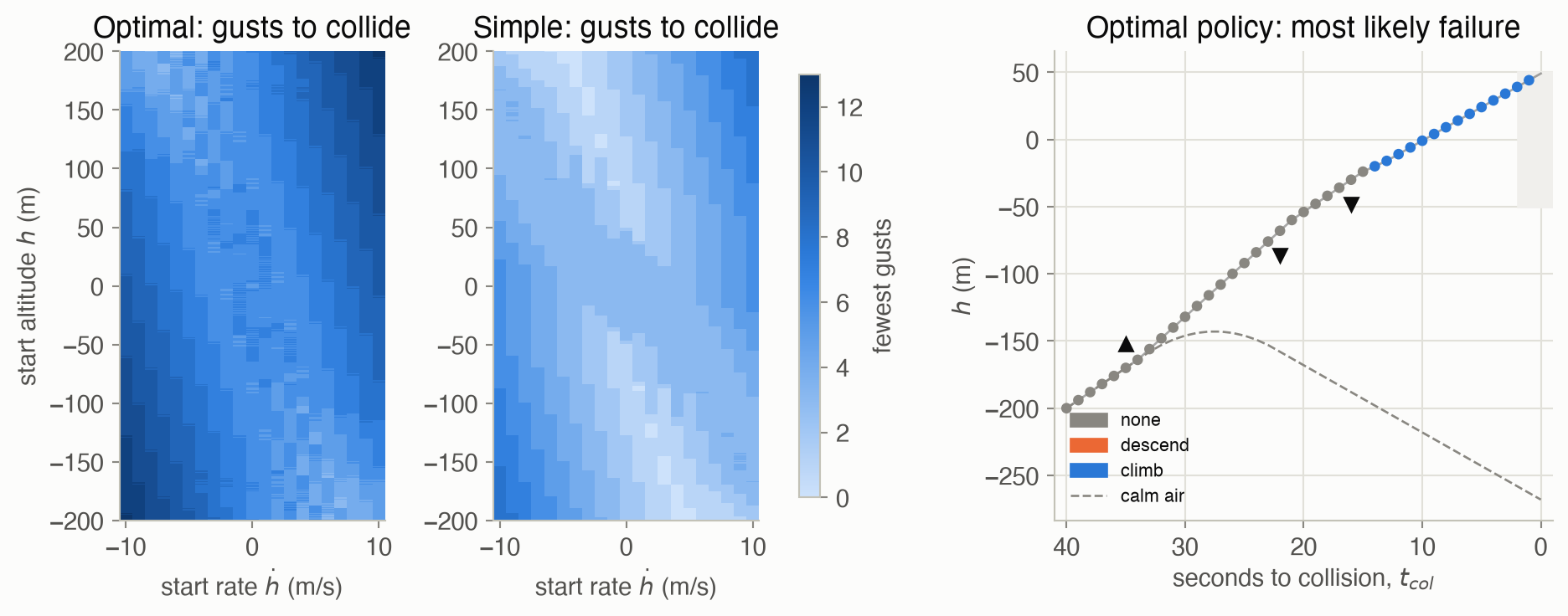
30 starts tie for the fewest gusts, 3. The figure shows the most surprising of them: the one whose calm-air encounter ends farthest from the intruder. It starts at \(h =\) -200 m, \(\dot h =\) 6 m/s, well below the intruder and climbing toward it. In calm air (dashed) the policy issues descend at 34 s and passes 268 m below. The adversary’s gusts, at 35 s, 22 s, 16 s before the encounter, turn that into a collision:
- An early upward gust speeds up the climb, so the aircraft now looks set to pass safely above the intruder. The policy stays silent instead of descending.
- Two downward gusts later slow the climb, until the path heads for the collision zone.
- The policy finally issues climb at 14 s. The advisory asks for 5 m/s, barely more than the 4 m/s the aircraft is already climbing at. The aircraft ends 49 m above the intruder, 1 m short of safe.
This is typical of what adversarial analysis produces: a concrete story that engineers can judge. Are three gusts, each half as likely as calm air, plausible at those moments? The path is \(2^{-3} = 1/8\) as likely as the calm-air path from the same start. The story also points at a specific weakness: late in the encounter, the strongest advisory adds little to a climb already under way. The simple policy, by contrast, fails in calm air from 2.0% of starts.
If a failure like this merits concern, the book lists the options: change the action space (here, stronger climb and descend advisories), the reward (cheaper advisory changes, as in Figure 8), the dynamics (a higher acceleration limit), or the solver, or don’t deploy.
Solved problems
Problem 1: how many simulations? A system’s failure probability is about \(10^{-5}\). How many direct simulations are needed for a relative standard error of 20%? How many failures would you expect to see?
TipSolution
The relative SE of a 0/1 estimate is \(\sqrt{(1-p)/(np)}\). Setting it to 0.2 gives \(n = (1-p)/(0.04\,p) \approx 2.5 \times 10^6\). That’s about \(np = 25\) failures. In general, relative error \(\approx 1/\sqrt{\text{failures}}\): 25 failures for 20%, 100 for 10%, whatever \(p\) is. Rarer events just take longer to produce those failures.
Problem 2: an importance weight. A proposal changes a coin with \(P(\text{heads}) = 0.1\) into one with \(P'(\text{heads}) = 0.5\). In 5 flips we see H, T, T, H, T. What is the importance weight of this sequence? If the event of interest is “at least 2 heads”, what does this one sample contribute to the estimate?
TipSolution
Heads contributes \(0.1/0.5 = 0.2\) and tails \(0.9/0.5 = 1.8\). The weight is \(0.2^2 \times 1.8^3 = 0.04 \times 5.832 = 0.233\). The event occurred, so the sample contributes \(1 \times 0.233 = 0.233\) to the average. For comparison, the true \(P(\ge 2 \text{ heads}) = 1 - 0.9^5 - 5(0.1)(0.9^4) \approx 0.081\). Samples with more heads get smaller weights, and samples with fewer heads (which rarely satisfy the event) get larger ones, and on average they balance.
Problem 3: the ideal proposal. A fair six-sided die is rolled. You want \(\mathbb{E}[f(X)]\) with \(f(x) = x\) if \(x \ge 5\) and 0 otherwise. What is the optimal proposal, and what does each of its samples contribute?
TipSolution
By Equation 5, \(P^*(x) \propto |f(x)|\,P(x)\): \(P^*(5) \propto 5/6\) and \(P^*(6) \propto 6/6\), so \(P^*(5) = 5/11\) and \(P^*(6) = 6/11\). A sample of 5 contributes \(f(5)\,P(5)/P^*(5) = 5 \times (1/6)/(5/11) = 11/6\). A sample of 6 contributes \(6 \times (1/6)/(6/11) = 11/6\). Every sample gives the exact answer \(\mathbb{E}[f] = (5 + 6)/6 = 11/6\): zero variance. Building \(P^*\) required knowing the answer, the normalizing sum 11/6, which is the catch.
Problem 4: a robust choice. In one state, action \(x\) has expected costs 1.0 under model A and 3.0 under model B, and action \(y\) has 1.8 under both. Which action does the nominal policy (model A only) choose, and which does robust dynamic programming choose? When is the robust choice a mistake?
TipSolution
The nominal policy picks \(x\) (1.0 < 1.8). Robust DP scores each action by its worst model: \(x \to 3.0\), \(y \to 1.8\), and picks \(y\). If model A is almost always right, the robust choice pays 0.8 extra nearly every time to insure against a rare case. Robust DP ignores how likely each model is; if the models’ probabilities are known, minimizing the expected cost over them (a belief over models, as in Part IV) can be the better choice.
Problem 5: when does the adversary give up? From some start, the most likely collision needs \(k\) gusts, each half as likely as calm air, and our only cost is 1 for a collision. For which \(\lambda\) does the adversary of Equation 8 choose the collision over the calm-air path? Check against the explorer’s start (60, 0), whose most likely collision needs 7 gusts.
TipSolution
The collision path’s log-likelihood is \(k \log 2\) below the calm path’s. The adversary prefers the collision when \(1 > \lambda k \log 2\), that is \(\lambda < 1/(k \log 2)\). For \(k = 7\): \(\lambda < 1/(7 \times 0.693) \approx 0.21\). In the explorer, the start (60, 0) collides for \(\lambda \le 0.1\) and stays safe at 0.3, as predicted. (Advisory changes add 0.01 each to the adversary’s reward, which barely moves the threshold.) At very small \(\lambda\) the adversary uses many more gusts than needed, because it also gains 0.01 for each advisory change it provokes.
Recap
- A performance metric is an expected trajectory score; additive scores are value functions (Equation 1, Equation 2). Why it matters: any policy evaluation method from Chapters 7–9 doubles as a validation tool. Here exact evaluation gave the true collision probability, 6.42e-04, against which every estimate was checked.
- Every simulated estimate needs an error bar, and rare events need relative ones (Equation 3). Why it matters: relative error is about one over the square root of the number of failures observed. 10,000 encounters with 5 collisions gave a 45% relative error.
- Importance sampling makes rare events common, then reweights (Equation 4, Equation 5). Why it matters: a proposal guided by an approximate risk-to-go matched about 63 times as many direct samples. An over-aggressive proposal was worse than none. Chapter 3’s likelihood weighting is the same idea.
- Policies are only as good as their models: stress-test them, and optimize against the worst case if needed (Equation 6). Why it matters: 80% pilot compliance made the optimal policy’s collision risk 6 times higher. Uncertainty about the model itself is the theme of Part III.
- Trade analysis separates dominated designs from real choices (Equation 7). Why it matters: the Pareto front shows what is achievable. Here every simple policy was beaten by an optimized one on both safety and alerts.
- Adversarial analysis turns validation into search for the most likely failure (Equation 8). Why it matters: it produces concrete, reviewable failure stories, like the late and too-weak climb above, and finds flaws, like the simple policy’s calm-air collisions, that random testing may take a long time to hit.
Cheat sheet & connections
| Name | Formula | Ref |
|---|---|---|
| Performance metric | \(f(\pi) = \mathbb{E}_\tau[f_{\text{traj}}(\tau)]\), \(P(\tau) = b(s_1)\prod_t T(s_{t+1} \mid s_t, \pi(s_t))\) | Equation 1 |
| Additive metric | \(f(\pi) = \sum_s f_{\text{state}}(s)\, b(s)\) by policy evaluation | Equation 2 |
| ★ Standard error | \(\hat\sigma/\sqrt n\); relative: \(\hat\sigma/(\hat\mu\sqrt n)\) | Equation 3 |
| ★ Importance sampling | \(\frac1n\sum_i f_{\text{traj}}(\tau^{(i)})\,P(\tau^{(i)})/P'(\tau^{(i)})\), \(\tau^{(i)} \sim P'\) | Equation 4 |
| Optimal proposal | \(P^* \propto |f_{\text{traj}}|\,P\); per step \(P'(\nu \mid s) \propto P(\nu)\,\hat U(s')\) | Equation 5 |
| Robust Bellman update | \(\max_a \min_i (R_i + \gamma \sum_{s'} T_i U_k)\) | Equation 6 |
| Pareto dominance | no worse on every metric, better on one | Equation 7 |
| Adversarial reward | \(-R(s, \pi(s)) + \lambda \log T(s' \mid s, \pi(s))\) | Equation 8 |
Common pitfalls
- Reporting a rare-event estimate without its relative error. Three failures in 10,000 trials is an estimate with an error bar about as wide as the estimate itself.
- A proposal that is too aggressive. Weights that vary over orders of magnitude give estimates that are unbiased on average but wrong in almost every run. Watch the effective sample size.
- A proposal that misses part of the failure space. If \(P'\) can’t produce some failures, the estimate is biased low, with no warning. Keep every outcome possible (the small constant in the guided proposal).
- Validating on the planning model only. A policy exploits its model’s assumptions, such as perfect compliance. Evaluate on models it wasn’t optimized for.
- Treating the most likely failure as the only failure. It is the single most probable failing path. Many less likely paths together can carry most of the risk.
Connections
- Ch 7 · Exact Solution Methods: policy evaluation and backward induction, used here for exact metrics and robust dynamic programming.
- Ch 3 · Inference: likelihood weighting, the same reweighting idea as importance sampling.
- Ch 4 · Parameter Learning: the Beta posterior behind the Bayesian interval.
- Ch 9 · Online Planning: search methods that can find adversarial trajectories in problems too large for dynamic programming.
- Ch 15 · Exploration and Exploitation: Part III begins, where the model itself must be learned.
- Appendix A · Mathematical Concepts: Monte Carlo and importance sampling from first principles. Appendix B · Probability Distributions: the Beta distribution behind the failure-probability intervals.