15 · Exploration and Exploitation
Part III — Model Uncertainty
Big picture
Where this chapter fits
Parts I and II assumed we know the model: the transition probabilities and the rewards. Part III drops that assumption. The agent must learn from its own experience, and this is reinforcement learning. Learning by acting raises a problem that planning never had. Every action both earns reward and produces information, and the two goals pull apart. This chapter studies that tension in its purest form, a problem with a single state: the multi-armed bandit. Chapters 16 and 17 carry the same ideas to problems with many states.
The question: when you don’t know which option is best, how much should you try options that look worse, to find out whether they really are?
The short answer: keep a belief about each option, and let its uncertainty drive exploration. Trying options at random (undirected exploration) is simple but keeps wasting pulls forever unless it is switched off on a schedule. Favoring options that might be best (directed exploration: optimism, upper confidence bounds, posterior sampling) spends exploration where it can pay off. With a finite number of pulls, the Bayes-optimal strategy can be computed exactly by dynamic programming over beliefs. It shows that how much to explore depends on how many pulls remain.
The key ideas at a glance
Bandits. Several slot machines (“arms”) pay 1 with unknown probabilities \(\theta_a\) and 0 otherwise. You have \(h\) pulls. Every pull earns a reward and teaches you about one arm. A/B tests, clinical trials, and ad placement all have this shape.
A belief per arm. Starting from a uniform prior, \(w\) wins and \(\ell\) losses give a \(\text{Beta}(w + 1, \ell + 1)\) posterior for an arm’s payoff probability (Chapter 4). Its mean, \((w + 1)/(w + \ell + 2)\), is the probability that the next pull wins. Its width says how much you still don’t know.
Exploitation versus exploration. The greedy choice pulls the arm with the highest posterior mean. It can lock onto a worse arm after an unlucky start and never find out. Exploration means sometimes pulling an arm that looks worse, to learn about it.
Undirected exploration ignores what you know: ε-greedy pulls a random arm with probability \(\varepsilon\); explore-then-commit pulls randomly for \(k\) steps, then goes greedy. With a fixed \(\varepsilon\), the wasted pulls never stop, so the loss (regret) grows in proportion to the number of pulls.
Directed exploration uses the uncertainty. Optimism under uncertainty scores each arm by an optimistic estimate: a high quantile of its posterior, or UCB1’s mean-plus-bonus. Thompson sampling draws a plausible payoff for each arm from its posterior and pulls the best draw. Arms that could plausibly be best get tried; arms that are clearly worse stop being tried.
Bayes-optimal exploration. The counts are a belief state, and a finite-horizon bandit is an MDP over those beliefs. Dynamic programming solves it exactly, but the number of belief states grows like \(h^{2n}\). It shows that the right amount of exploration depends on the pulls remaining: with one pull left, greedy is optimal.
Vocabulary
| Term | Plain meaning |
|---|---|
| Arm \(a\), payoff probability \(\theta_a\) | An option, and its unknown chance of paying 1 |
| Horizon \(h\) | The number of pulls available |
| Counts \(w_a\), \(\ell_a\) | Wins and losses observed on arm \(a\) |
| Posterior \(\text{Beta}(w_a + 1, \ell_a + 1)\) | The belief about \(\theta_a\) after those counts, from a uniform prior |
| \(\rho_a\) | Posterior probability that the next pull of arm \(a\) wins |
| Greedy arm | An arm with the highest \(\rho_a\) |
| Regret | Expected reward lost compared with always pulling the best arm |
| Undirected / directed exploration | Exploring blindly, or guided by the uncertainty |
| Optimism under uncertainty | Acting as if each arm were as good as the data plausibly allow |
| Thompson (posterior) sampling | Pull the arm whose sampled payoff probability is highest |
| Bayes-optimal policy | The best possible strategy for a given prior and horizon |
After this chapter you can
- Maintain Beta beliefs for a Bernoulli bandit and compute each arm’s win probability.
- Implement ε-greedy, explore-then-commit, softmax, quantile, UCB1 and Thompson sampling, and tune them.
- Explain why fixed undirected exploration has regret that grows linearly, and why directed methods do much better over long horizons.
- Compute the Bayes-optimal strategy for a small bandit by dynamic programming over belief states, and explain why it depends on the pulls remaining.
Intuition
TipAnalogy
You’ve moved to a new town with three coffee shops. One visit tells you little: even a good shop has off days.
- Pure exploitation: after one great latte at shop A, you go there forever and never learn that shop C is better.
- Pure exploration: you rotate among all three forever, drinking plenty of mediocre coffee long after you could have known better.
- Sensible: try each a few times. Keep going back to a shop that might be the best, and stop visiting one that clearly isn’t.
- How long you’ll live there matters. If you’re leaving next week, stick with what’s good now; if you’re staying ten years, explore more.
Our running example is a newsletter testing three headlines. Each reader who sees a headline clicks (1) or doesn’t (0). The click rates are A: 0.35, B: 0.50, C: 0.55, but the editor doesn’t know them. Every reader is one pull of a three-armed bandit.
Counting wins is a belief
After 5 clicks from 8 readers, a headline’s click rate could be anything from about 0.3 to 0.9. The Beta posterior summarizes exactly that: \(\text{Beta}(6, 4)\), with mean \(6/10 = 0.6\). After 50 clicks from 80 readers, the mean is similar, but the posterior is much narrower. The mean says which headline looks best; the width says how much to trust that (Figure 4). See Equation 2.
Greedy gets stuck
The greedy editor always shows the headline with the best mean so far. If the best headline has a couple of unlucky first readers, its mean drops. Greedy then never shows it again, and never finds out. Over 1,000 readers of randomly chosen three-headline tests, greedy loses 33.3 clicks on average compared with always showing the best headline. That loss is its regret. See Equation 1.
Random exploration never stops paying
ε-greedy shows a random headline to 10% of readers. That rescues it from getting stuck, but it keeps showing bad headlines to 10% of readers forever. Its regret after 1,000 readers is 32.4, still growing in a straight line. Decaying \(\varepsilon\) over time helps: 15.5. See Equation 3.
Be optimistic about what you haven’t seen
Score each headline by how good it could plausibly be: a high quantile of its posterior, or its mean plus a bonus that shrinks as it gets shown more. A rarely shown headline has a wide posterior and a high optimistic score, so it gets tried. A headline that has been shown often and is clearly worse has a narrow posterior and a low score, so it stops being tried. With the 99% quantile, regret after 1,000 readers is 7.0. See Equation 5 and Equation 6.
Sample a plausible world
Thompson sampling draws one plausible click rate for each headline from its posterior, and shows the headline with the highest draw. A headline is shown as often as it is likely to be the best. There is nothing to tune. Its regret is 10.0 after 1,000 readers (Figure 5). See Equation 7.
How long is the game?
With only a few readers left, exploring is pointless: there’s no time to use what you’d learn. Take headline A with 5 clicks from 8 readers and headline B with 1 click from 2. A looks better (mean 0.60 against 0.50). The Bayes-optimal choice is A while fewer than 19 readers remain, and B, to learn about it, when 19 or more remain. In short tests, even plain greedy is close to optimal. Over 10 pulls of a two-armed bandit it loses 0.66, against the optimum’s 0.64. See Equation 8.
Formalism
Bandit problems and regret
A Bernoulli bandit has \(n\) arms. Pulling arm \(a\) pays 1 with probability \(\theta_a\) and 0 otherwise, independently each time; we have \(h\) pulls (ADM §15.1). It is an \(h\)-step MDP with one state, \(n\) actions and an unknown reward function. How well a strategy does is measured against an oracle that knows the best arm:
\[ \text{regret}(h) = h\,\theta^* - \mathbb{E}\Big[\sum_{t=1}^h r_t\Big] = \mathbb{E}\Big[\sum_{t=1}^h \big(\theta^* - \theta_{a_t}\big)\Big], \qquad \theta^* = \max_a \theta_a \tag{1}\]
In words. Regret is the reward you gave up by not knowing which arm is best: each pull of a worse arm costs the gap between its payoff probability and the best one.
Term by term.
- \(a_t\) is the arm pulled at step \(t\), and \(r_t\) the reward it paid.
- The second form counts only the gaps, which removes the luck of the individual wins and losses. The simulations on this page use it.
- Bayes regret also averages over bandits drawn from a prior. With \(\theta_a \sim U(0, 1)\) for two arms, \(\mathbb{E}[\theta^*] = 2/3\), so the oracle earns \(2h/3\).
Why it holds. \(\mathbb{E}[r_t \mid a_t] = \theta_{a_t}\), so the expected total reward is \(\mathbb{E}[\sum_t \theta_{a_t}]\). Subtracting it from \(h\theta^*\) gives the sum of gaps.
This book’s chapter doesn’t define regret, but it is the standard yardstick for bandit algorithms (T. Lattimore and C. Szepesvári, Bandit Algorithms, 2020).
Bayesian model estimation
With a uniform prior \(\text{Beta}(1, 1)\), arm \(a\)’s posterior after \(w_a\) wins and \(\ell_a\) losses is \(\text{Beta}(w_a + 1, \ell_a + 1)\) (ADM §15.2; Chapter 4). The probability that its next pull wins is
\[ \rho_a = P(\text{win}_a \mid w_a, \ell_a) = \int_0^1 \theta\, \text{Beta}(\theta \mid w_a + 1, \ell_a + 1)\, d\theta = \frac{w_a + 1}{w_a + \ell_a + 2} \tag{2}\]
In words. Add one imaginary win and one imaginary loss to the counts, then take the win fraction.
Term by term.
- The integral averages the win probability \(\theta\) over everything we believe about it.
- The mean of \(\text{Beta}(\alpha, \beta)\) is \(\alpha/(\alpha + \beta)\), which gives the fraction.
- The “+1” and “+2” come from the prior. With no data, \(\rho_a = 1/2\). This is Laplace’s rule of succession.
Why it holds. By Bayes’ rule, the posterior is proportional to prior × likelihood \(= 1 \times \theta^{w}(1 - \theta)^{\ell}\), which is a \(\text{Beta}(w + 1, \ell + 1)\) density.
Updating is counting: a win adds 1 to \(w_a\), a loss adds 1 to \(\ell_a\).
Undirected exploration
ε-greedy pulls a uniformly random arm with probability \(\varepsilon\) and a greedy arm, \(\arg\max_a \rho_a\), otherwise. Explore-then-commit pulls random arms for the first \(k\) steps, then greedy ones (ADM §15.3). Because a constant \(\varepsilon\) explores as much at the end as at the start, it is often decayed:
\[ P(a) = \frac{\varepsilon_t}{n} + (1 - \varepsilon_t)\, \mathbb{1}\big[a = \arg\max_{a'} \rho_{a'}\big], \qquad \varepsilon_{t+1} = \alpha\, \varepsilon_t \tag{3}\]
In words. Usually take the best-looking arm; occasionally take any arm at random, and do that less and less as time goes on.
Term by term.
- The random choice may land on the greedy arm too, so the greedy arm’s probability is \(1 - \varepsilon_t + \varepsilon_t/n\).
- \(\alpha \in (0, 1)\), close to 1, is the decay factor.
- Ties for the greedy arm are split evenly.
Why it holds. With a fixed \(\varepsilon\), a worse arm with gap \(\Delta\) is pulled at least \(\varepsilon/n\) of the time, so regret grows at least as \(h\,\varepsilon\,\bar\Delta\), where \(\bar\Delta\) is the average gap over the arms: linearly in \(h\). Decaying \(\varepsilon\) removes that floor.
Directed exploration
Softmax pulls arm \(a\) with probability proportional to \(\exp(\lambda \rho_a)\) (ADM §15.4):
\[ P(a) = \frac{\exp(\lambda \rho_a)}{\sum_{a'} \exp(\lambda \rho_{a'})} \tag{4}\]
In words. Better-looking arms are pulled more often, but every arm keeps some chance, graded by how good it looks.
Term by term. The precision \(\lambda \ge 0\) runs from uniform (\(\lambda = 0\)) to greedy (\(\lambda \to \infty\)). Multiplying \(\lambda\) by a factor slightly above 1 after each pull reduces exploration over time. Softmax uses only the means, not the uncertainty: two arms with equal means get equal probability, however many times each was pulled.
Quantile exploration is optimistic in proportion to the uncertainty:
\[ a = \arg\max_a\ F^{-1}_{\text{Beta}(w_a + 1,\, \ell_a + 1)}(\alpha) \tag{5}\]
In words. Score each arm by the payoff probability it exceeds only with probability \(1 - \alpha\): an optimistic but plausible value.
Term by term. \(F^{-1}(\alpha)\) is the posterior’s \(\alpha\)-quantile. For \(\alpha > 0.5\) it lies above the median, and further above for wider posteriors, so rarely tried arms get a boost. Larger \(\alpha\) means more optimism.
UCB1 uses a simple bonus instead of the exact quantile:
\[ a = \arg\max_a\ \rho_a + c \sqrt{\frac{\log N}{N(a)}} \tag{6}\]
In words. Mean plus a bonus that is large for arms pulled rarely compared with the total.
Term by term.
- \(N(a)\) counts arm \(a\)’s pulls and \(N = \sum_a N(a)\). Here we use the Beta pseudocounts, \(N(a) = w_a + \ell_a + 2\), so untried arms need no special case.
- \(c \ge 0\) sets the strength of exploration; \(c = 0\) is greedy.
- \(\log N\) grows slowly, so an arm that is not pulled sees its bonus creep up until it is tried again: every arm is revisited, but ever more rarely.
Why it holds. The bonus is the width of a confidence interval (from Hoeffding’s inequality) around the observed mean. An arm is pulled only if its interval reaches above the best arm’s mean, which a worse arm’s interval stops doing after about \(\log h / \Delta^2\) pulls. This keeps the regret growing only logarithmically (P. Auer et al., Machine Learning, 2002). UCB1 appeared as the exploration rule of Monte Carlo tree search in Chapter 9.
Thompson sampling (posterior sampling) needs no parameter:
\[ \tilde\theta_a \sim \text{Beta}(w_a + 1, \ell_a + 1),\quad a = \arg\max_a \tilde\theta_a; \qquad P(a) = P\big(\theta_a = \max_{a'} \theta_{a'} \mid \text{data}\big) \tag{7}\]
In words. Imagine one plausible world by sampling each arm’s payoff probability from its posterior, then act optimally in that world. Each arm is pulled with exactly the probability that it is the best one.
Term by term.
- Each \(\tilde\theta_a\) is one draw from arm \(a\)’s posterior.
- The probability of choosing \(a\) is \(\int_0^1 p_a(x) \prod_{a' \neq a} F_{a'}(x)\, dx\): arm \(a\)’s draw is \(x\) and every other draw is below it. The code computes it this way for exact evaluation. The integrand is a polynomial, so Gauss–Legendre quadrature gets it exactly.
Why it holds. The second form follows from the first: since the draws are from the posterior, the arm with the largest draw is distributed like the arm that is actually best, given the data (W. R. Thompson, Biometrika, 1933).
Bayes-optimal exploration
The counts \((w_1, \ell_1, \ldots, w_n, \ell_n)\) are a belief state, and each pull moves it to one of two next beliefs. With \(r\) pulls remaining, the optimal expected reward satisfies (ADM §15.5)
\[ Q^*_r(w, \ell, a) = \rho_a\big(1 + U^*_{r-1}(\ldots, w_a + 1, \ell_a, \ldots)\big) + (1 - \rho_a)\, U^*_{r-1}(\ldots, w_a, \ell_a + 1, \ldots), \qquad U^*_r = \max_a Q^*_r,\quad U^*_0 = 0 \tag{8}\]
In words. Pulling arm \(a\) wins with probability \(\rho_a\), earning 1 and a belief with one more win; otherwise it earns nothing and a belief with one more loss. Either way, continue optimally.
Term by term.
- \(\rho_a\) from Equation 2 is both the chance of the reward and the chance of that belief update.
- The first \(U^*\) holds the value after a win, the second after a loss. Their difference is what the pull teaches: the value of information.
- With \(r = 1\), both \(U^*_0\) terms are 0, and \(Q^*_1 = \rho_a\): the last pull is greedy.
- Backward induction from \(r = 0\) solves it exactly. With \(n\) arms and horizon \(h\) there are \(\binom{h + 2n}{2n}\) belief states, \(O(h^{2n})\): fine for two arms and dozens of pulls, hopeless for many arms. For the infinite-horizon discounted version, the Gittins index gives an optimal policy from a per-arm lookup table (J. C. Gittins, JRSS B, 1979).
Why it holds. It is the Bellman optimality equation (Chapter 7) for the MDP whose states are beliefs, whose transitions are Bayesian updates, and whose rewards are the expected payoffs. The same code, with the \(\max\) replaced by an average over a strategy’s action probabilities, evaluates any strategy exactly.
Exploration with many states
In a general MDP with unknown dynamics, the loop is the same (ADM §15.6). The agent chooses \(a\) from its current model and state, the environment returns \(s'\) and \(r\), the model is updated with \((s, a, r, s')\), and the agent moves on to \(s'\). What changes is the model: counts of transitions and rewards per state and action (Chapter 16), or action values learned directly (Chapter 17). The exploration strategies of this chapter apply per state, and so does the tension between exploring and exploiting. In addition, a state may have to be reached before it can be explored.
Worked example
Six strategies, one belief
Headline A has 5 clicks from 8 readers; headline B has 1 click from 2. What does each strategy do next?
- Posteriors: A is \(\text{Beta}(6, 4)\) with \(\rho_A = 6/10 = 0.6\); B is \(\text{Beta}(2, 2)\) with \(\rho_B = 2/4 = 0.5\).
- 90% quantiles: A 0.790, B 0.804. B’s wider posterior reaches higher.
- UCB1 scores with \(c = 0.5\), \(N = 10 + 4 = 14\) pseudocounts: A \(0.6 + 0.5\sqrt{\log 14 / 10} =\) 0.857, B \(0.5 + 0.5\sqrt{\log 14 / 4} =\) 0.906.
| Strategy | P(pull A) | P(pull B) |
|---|---|---|
| greedy | 1.000 | 0.000 |
| ε-greedy, ε = 0.2 | 0.900 | 0.100 |
| softmax, λ = 10 | 0.731 | 0.269 |
| quantile, α = 0.9 | 0.000 | 1.000 |
| UCB1, c = 0.5 | 0.000 | 1.000 |
| Thompson sampling | 0.636 | 0.364 |
- Greedy and ε-greedy favor A, the higher mean.
- Quantile and UCB1 pick B for sure: its uncertainty lifts its optimistic score above A’s.
- Softmax leans toward A but keeps a real chance for B.
- Thompson sampling pulls A with the posterior probability that A is the better headline.
The value of looking
What would the Bayes-optimal editor do? With one reader left, \(Q^*_1 = \rho\): 0.60 for A, 0.50 for B. Pick A. With two readers left, work out B by hand. After a click on B, B’s mean becomes \(3/5 = 0.6\), tied with A, so the last reader is worth 0.6. After no click, B’s mean drops to \(2/5\) and A is best at 0.6. So
\[Q^*_2(B) = 0.5\,(1 + 0.6) + 0.5\,(0.6) = 1.1,\]
while \(Q^*_2(A) =\) 1.2: pulling A now and A again. With so few readers left, learning about B can’t pay. But the gap narrows as more readers remain:
| Readers left \(r\) | 1 | 2 | 5 | 10 | 20 | 30 |
|---|---|---|---|---|---|---|
| \(Q^*_r(A)\) | 0.600 | 1.200 | 3.022 | 6.137 | 12.495 | 18.934 |
| \(Q^*_r(B)\) | 0.500 | 1.100 | 2.967 | 6.115 | 12.499 | 18.949 |
From 19 readers left on (checked up to 30), B is the better pull: there is enough time left for what B might reveal to pay off.
Interactive
Bandit playground
Follow one run of each strategy on the headline test (click rates 0.35, 0.50, 0.55). The top chart shows each headline’s posterior after the chosen number of readers; the bottom shows each strategy’s regret so far, with the selected one highlighted.
This is one run, so luck matters: rerunning with another seed would reorder the strategies. Figure 5 averages over 2,000 random tests.
When should the optimal editor explore?
Headline B has the counts chosen below; headline A’s counts vary across the grid. Each cell shows whether the Bayes-optimal editor shows A or B next, for the chosen number of readers left. The dashed line marks where A’s and B’s posterior means are equal: greedy shows B only below and to the right of it, where A’s mean is lower.
Algorithms & code
Beliefs and strategies
def posterior_mean(w: Array, l: Array) -> Array:
    """rho_a = P(win | w_a, l_a) = (w_a + 1) / (w_a + l_a + 2) (eq. 15.1)."""
    return (w + 1) / (w + l + 2)

class EpsilonGreedy(Strategy):
    """A random arm with probability eps (decayed as eps * decay^t,
    eq. 15.2), otherwise a greedy one."""

    def __init__(self, eps, decay=1.0):
        self.eps, self.decay = eps, decay

    def probs(self, w, l, t):
        eps = self.eps * self.decay**t
        n = w.shape[-1]
        return eps / n + (1 - eps) * argmax_split(posterior_mean(w, l))

class ExploreThenCommit(Strategy):
    """Uniformly random arms for the first k pulls, then greedy."""

    def __init__(self, k):
        self.k = k

    def probs(self, w, l, t):
        if t < self.k:
            return np.full(w.shape, 1 / w.shape[-1])
        return argmax_split(posterior_mean(w, l))

class Softmax(Strategy):
    """P(a) proportional to exp(lam * rho_a), with the precision growing
    as lam * factor^t."""

    def __init__(self, lam, factor=1.0):
        self.lam, self.factor = lam, factor

    def probs(self, w, l, t):
        z = self.lam * self.factor**t * posterior_mean(w, l)
        z = np.exp(z - z.max(axis=-1, keepdims=True))  # subtract max: no overflow
        return z / z.sum(axis=-1, keepdims=True)

class Quantile(Strategy):
    """The arm whose posterior has the highest alpha-quantile: optimism
    under uncertainty when alpha > 0.5."""

    def __init__(self, alpha):
        self.alpha = alpha

    def probs(self, w, l, t):
        return argmax_split(stats.beta.ppf(self.alpha, w + 1, l + 1))

class UCB1(Strategy):
    """The arm maximizing rho_a + c sqrt(log N / N_a) (eq. 15.3), with
    the Beta pseudocounts N_a = w_a + l_a + 2 and N = sum_a N_a."""

    def __init__(self, c):
        self.c = c

    def probs(self, w, l, t):
        Na = w + l + 2
        N = Na.sum(axis=-1, keepdims=True)
        return argmax_split(posterior_mean(w, l) + self.c * np.sqrt(np.log(N) / Na))

class Thompson(Strategy):
    """Posterior (Thompson) sampling: draw theta_a from each posterior and
    pull the arm with the largest draw. Its probabilities are
    P(a) = integral of pdf_a(x) prod_{b != a} cdf_b(x) dx."""

    def probs(self, w, l, t):
        x = _X[:, None]                                # (nodes, 1): broadcasts over arms
        pdf = stats.beta.pdf(x, w[..., None, :] + 1, l[..., None, :] + 1)
        cdf = stats.beta.cdf(x, w[..., None, :] + 1, l[..., None, :] + 1)
        # prod over the other arms = prod over all arms / own cdf, done in
        # logs; an arm's own cdf can be 0 only where its pdf is also 0.
        with np.errstate(divide="ignore", invalid="ignore"):
            others = np.exp(np.log(cdf).sum(axis=-1, keepdims=True) - np.log(cdf))
        others = np.nan_to_num(others)
        p = (_WX[:, None] * pdf * others).sum(axis=-2)
        return p / p.sum(axis=-1, keepdims=True)

    def act(self, w, l, t, rng):
        return rng.beta(w + 1, l + 1).argmax(axis=-1)

def simulate(theta: Array, strategy: Strategy, h: int, rng):
    """Run a strategy on bandits side by side for h pulls.

    theta has shape (m, n_arms): row i is bandit i's win probabilities.
    Returns (actions, rewards), each of shape (m, h), and the final
    counts (w, l).
    """
    m, n = theta.shape
    w, l = np.zeros((m, n), dtype=int), np.zeros((m, n), dtype=int)
    rows = np.arange(m)
    A, R = np.zeros((m, h), dtype=int), np.zeros((m, h), dtype=int)
    for t in range(h):
        a = strategy.act(w, l, t, rng)
        r = (rng.random(m) < theta[rows, a]).astype(int)
        w[rows, a] += r                      # paired indexing: one arm per row
        l[rows, a] += 1 - r
        A[:, t], R[:, t] = a, r
    return A, R, (w, l)
using Random, Statistics
import Distributions
# Belief: wins w[a] and losses l[a]; posterior Beta(w + 1, l + 1); ρ = (w + 1)/(w + l + 2).
posterior_mean(w, l) = (w .+ 1) ./ (w .+ l .+ 2)
greedy(w, l, rng) = rand(rng, findall(==(maximum(posterior_mean(w, l))), posterior_mean(w, l))) # random tie-break
# Each strategy maps (w, l, t, rng) to an arm (1-based).
epsilon_greedy(ε; decay = 1.0) = (w, l, t, rng) -> rand(rng) < ε * decay^t ? rand(rng, eachindex(w)) : greedy(w, l, rng)
quantile_rule(α) = (w, l, t, rng) -> argmax([Distributions.quantile(Distributions.Beta(w[a] + 1, l[a] + 1), α) for a in eachindex(w)])
function ucb1(c)
return function (w, l, t, rng)
Na = w .+ l .+ 2 # Beta pseudocounts per arm
argmax(posterior_mean(w, l) .+ c .* sqrt.(log(sum(Na)) ./ Na))
end
end
thompson() = (w, l, t, rng) -> argmax([rand(rng, Distributions.Beta(w[a] + 1, l[a] + 1)) for a in eachindex(w)])
# Run one strategy on one bandit for h pulls; return the regret (sum of gaps).
function run_bandit(θ, strategy, h, rng)
w, l, regret = zeros(Int, length(θ)), zeros(Int, length(θ)), 0.0
for t in 0:h-1
a = strategy(w, l, t, rng)
rand(rng) < θ[a] ? (w[a] += 1) : (l[a] += 1) # update the belief by counting
regret += maximum(θ) - θ[a]
end
return regret
end
# Average regret over 300 random three-armed bandits, 1,000 pulls each.
rng = MersenneTwister(0)
bandits = [rand(rng, 3) for _ in 1:300]
for (name, s) in (("ε-greedy 0.1", epsilon_greedy(0.1)), ("quantile 0.99", quantile_rule(0.99)),
("UCB1 0.5", ucb1(0.5)), ("Thompson", thompson()))
println(rpad(name, 14), round(mean(run_bandit(θ, s, 1000, rng) for θ in bandits); digits = 1))
end
@assert mean(run_bandit(θ, thompson(), 1000, rng) for θ in bandits) <
mean(run_bandit(θ, epsilon_greedy(0.1), 1000, rng) for θ in bandits)Exact evaluation and the Bayes-optimal strategy
def evaluate(strategy, n: int, h: int, optimal=False):
    """Exact expected total reward of a strategy over h pulls, averaged
    over bandits drawn from the uniform prior (theta_a ~ U(0, 1)).

    Backward induction over belief states (the counts), one layer of
    total t at a time. With optimal=True it computes the Bayes-optimal
    value instead (eq. 15.6), ignoring `strategy`. Returns the value at
    the start (all counts 0).
    """
    V = np.zeros((h + 1,) * (2 * n))           # V[w_1, l_1, ..., w_n, l_n]
    for t in range(h - 1, -1, -1):
        S = _layer(t, n)                       # (m, 2n)
        w, l = S[:, 0::2], S[:, 1::2]          # wins and losses, (m, n)
        rho = posterior_mean(w, l)
        Q = np.zeros(w.shape)
        for a in range(n):
            win, loss = S.copy(), S.copy()
            win[:, 2 * a] += 1
            loss[:, 2 * a + 1] += 1
            # V[tuple(columns)] looks up one value per row of counts.
            Q[:, a] = (rho[:, a] * (1 + V[tuple(win.T)])
                       + (1 - rho[:, a]) * V[tuple(loss.T)])
        if optimal:
            V[tuple(S.T)] = Q.max(axis=1)
        else:
            V[tuple(S.T)] = (strategy.probs(w, l, t) * Q).sum(axis=1)
    return V[(0,) * (2 * n)]

def optimal_values(r_max: int, k_max: int):
    """Bayes-optimal values of a two-armed bandit with r pulls left.

    Returns U with U[r, w1, l1, w2, l2] for r = 0..r_max and counts up
    to k_max (states whose next counts would exceed k_max are left 0,
    so keep k_max >= largest total count + r). Q values for the two arms
    are then q_values(U, r, ...). Recursion (eq. 15.6):
      U_r(c) = max_a [rho_a (1 + U_{r-1}(c + win_a))
                      + (1 - rho_a) U_{r-1}(c + loss_a)].
    """
    K = k_max + 1
    U = np.zeros((r_max + 1, K, K, K, K))
    for r in range(1, r_max + 1):
        U[r, :-1, :-1, :-1, :-1] = np.max(q_values(U, r), axis=0)
    return U

def q_values(U, r):
    """Q[a, w1, l1, w2, l2] with r pulls left, for counts below k_max
    (the arrays are one shorter on each axis than U's count axes)."""
    K = U.shape[1]
    w1, l1, w2, l2 = np.meshgrid(*(np.arange(K - 1),) * 4, indexing="ij")
    prev = U[r - 1]
    rho1, rho2 = posterior_mean(w1, l1), posterior_mean(w2, l2)
    # Slicing shifts one count by 1: prev[1:, :-1, :-1, :-1] is
    # U_{r-1} at (w1 + 1, l1, w2, l2), a win for arm 1.
    q1 = rho1 * (1 + prev[1:, :-1, :-1, :-1]) + (1 - rho1) * prev[:-1, 1:, :-1, :-1]
    q2 = rho2 * (1 + prev[:-1, :-1, 1:, :-1]) + (1 - rho2) * prev[:-1, :-1, :-1, 1:]
    return np.array([q1, q2])
# Bayes-optimal value of a two-armed Bernoulli bandit with r pulls left, from counts
# c = (w1, l1, w2, l2), by memoized recursion on eq. 15.6.
const memo = Dict{Tuple{Int,NTuple{4,Int}},Float64}()
function U(r, c)
r == 0 && return 0.0
get!(memo, (r, c)) do # compute once per (r, c), then reuse
best = -Inf
for a in 1:2
w, l = c[2a-1], c[2a]
ρ = (w + 1) / (w + l + 2)
win = Base.setindex(c, w + 1, 2a - 1) # a copy of the tuple with one count changed
loss = Base.setindex(c, l + 1, 2a)
best = max(best, ρ * (1 + U(r - 1, win)) + (1 - ρ) * U(r - 1, loss))
end
best
end
end
@assert U(1, (5, 3, 1, 1)) ≈ 0.6 # last pull: greedy
@assert U(2, (0, 0, 0, 0)) ≈ 13 / 12
v30 = U(30, (0, 0, 0, 0))
println("Bayes-optimal reward over 30 pulls: ", round(v30; digits = 4), " (oracle 20)")
@assert 18.9 < v30 < 18.95
NoteReading the Julia code (for Python programmers)
(w, l, t, rng) -> ...is an anonymous function, likelambda.epsilon_greedy(0.1)returns one, so strategies are just functions.findall(==(m), v)returns the indices wherevequalsm;==(m)is a one-argument function (a curried comparison).get!(memo, key) do ... endreturns the cached value, or runs the block, stores its result and returns it. It is the idiom for memoization, likefunctools.cache.Base.setindex(c, v, i)(no!) returns a new tuple with elementireplaced: tuples are immutable, like Python’s.c[2a-1]:2ameans2 * a, and indices start at 1, so arma’s wins and losses sit at positions2a - 1and2a.
Run them
theta = np.random.default_rng(3).random((500, 3))       # 500 random three-armed bandits
A, R, (w, l) = simulate(theta, Thompson(), 1000, np.random.default_rng(4))
regret_ts = (theta.max(axis=1)[:, None] - np.take_along_axis(theta, A, axis=1)).sum(axis=1)

exact_greedy = evaluate(Greedy(), n=2, h=30)             # exact, over the uniform prior
exact_best = evaluate(None, n=2, h=30, optimal=True)
Thompson sampling, 1,000 pulls: regret 10.1 ± 0.4
30 pulls, two arms (exact): greedy 18.778, Bayes-optimal 18.920, oracle 20Results
Beliefs narrow where the pulls go
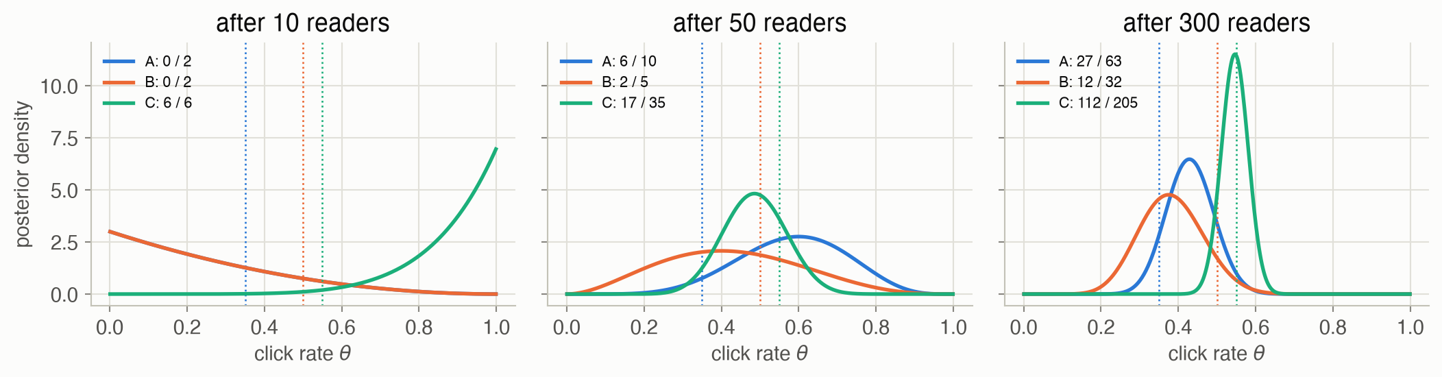
This run shows how luck steers exploration:
- Early luck gets a headline shown. The weakest headline, A, drew 6 clicks from its first 10 readers, so its posterior looked promising, and Thompson sampling kept showing it until its mean came down.
- Early bad luck gets a headline neglected. B, truly better than A, started with 0 clicks from 2 readers. After 300 readers it has been shown only 32 times, and its posterior is the widest. It is not written off, though: its wide posterior still gives it a chance of being sampled highest.
- The best headline wins most readers. C was shown to 205 of the 300, and its posterior has narrowed around its true click rate.
A single run is noisy; Figure 5 averages over thousands.
Undirected versus directed exploration over 1,000 pulls
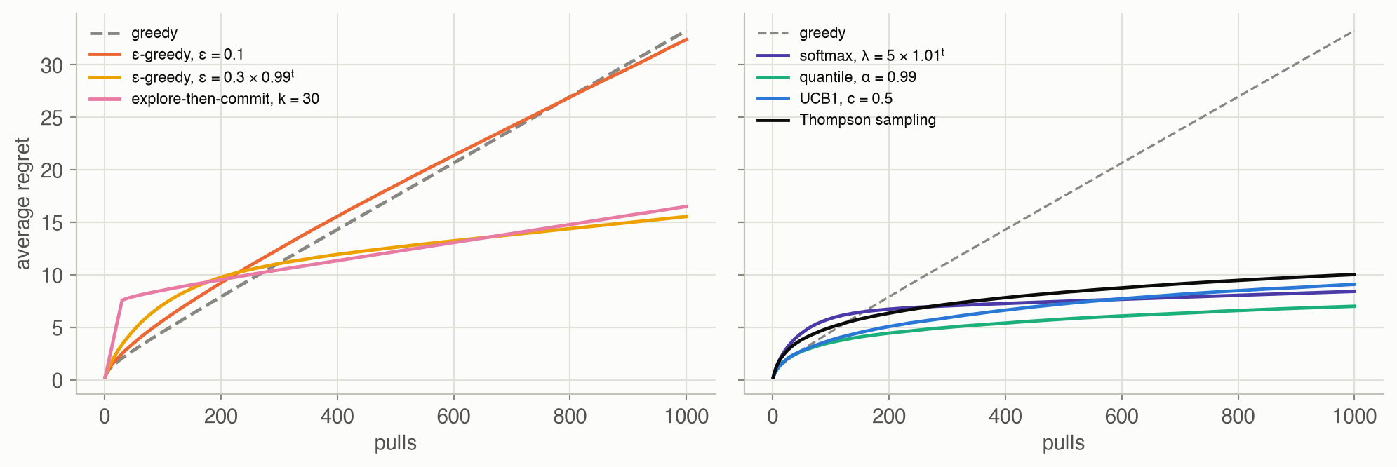
| Strategy | Regret after 1,000 pulls |
|---|---|
| greedy | 33.3 ± 1.7 |
| ε-greedy, ε = 0.1 | 32.4 ± 0.4 |
| ε-greedy, ε = 0.3 × 0.99ᵗ | 15.5 ± 0.5 |
| explore-then-commit, k = 30 | 16.5 ± 0.7 |
| softmax, λ = 5 × 1.01ᵗ | 8.4 ± 0.2 |
| quantile, α = 0.99 | 7.0 ± 0.2 |
| UCB1, c = 0.5 | 9.1 ± 0.2 |
| Thompson sampling | 10.0 ± 0.2 |
- Greedy and fixed ε-greedy grow almost in a straight line. Greedy gets stuck on a worse arm in a fraction of the bandits and pays the gap on every pull. ε-greedy pays for its random pulls forever.
- Decaying ε and explore-then-commit stop exploring. They do better, but depend on a schedule that must be tuned to the horizon.
- The directed strategies end between 7.0 and 10.0. Their curves bend over: each additional pull costs less and less, consistent with the logarithmic growth that theory predicts for UCB1 and Thompson sampling. Thompson sampling needed no tuning; the others’ parameters were picked from a handful of values.
Tuning, exactly, at short horizons
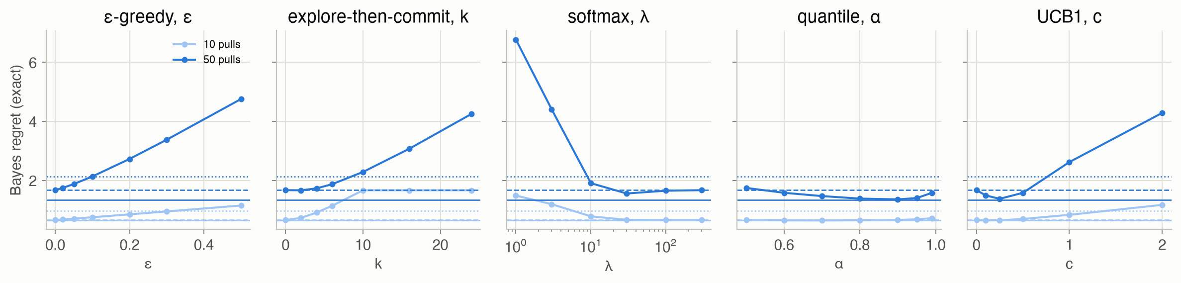
These values are exact: dynamic programming over belief states averages over every possible bandit and every possible sequence of wins and losses, with no simulation noise.
- Short horizons favor exploiting. Over 10 pulls, greedy’s regret is 0.661, against the Bayes-optimal 0.645. Over 50 pulls, greedy’s regret is 1.67 against 1.34.
- Thompson sampling explores too much for short games: 0.962 over 10 pulls and 2.13 over 50, worse than greedy at both. It doesn’t know how many pulls are left, and learning is worth less when little time remains to use it. Over 1,000 pulls it was far better than greedy (10.0 against 33.3), though the tuned directed strategies did better still.
- The best parameters over 50 pulls were ε = 0.0 (plain greedy), k = 2, λ = 30, α = 0.9 and c = 0.25. The best tuned strategy reached 1.36, close to the optimum.
The Bayes-optimal strategy explores more when more time remains
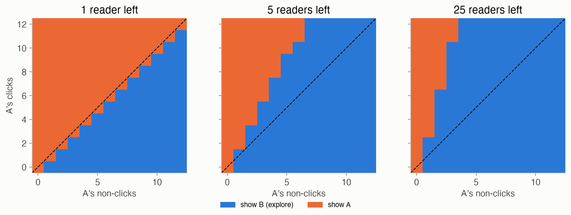
With one reader left, the optimal editor is greedy: it shows untried B only when A’s mean is below 0.5. With 25 readers left, it tries B even when A’s mean is as high as 0.73, as long as A’s record is short. Learning that B is excellent would pay for many readers. When A has a long, good record, trying B is not worth it at any horizon shown.
Solved problems
Problem 1: a posterior by hand. A drug trial arm has 7 successes and 2 failures. With a uniform prior, what is the posterior, and the probability that the next patient succeeds? What would it be after 70 successes and 20 failures?
TipSolution
The posterior is \(\text{Beta}(8, 3)\), so \(\rho = 8/11 \approx 0.727\). After 70 and 20 it is \(\text{Beta}(71, 21)\) with \(\rho = 71/92 \approx 0.772\). The means approach the observed rate, 7/9 ≈ 0.778, as the prior’s two pseudo-observations matter less. The posterior’s standard deviation falls from about 0.13 to about 0.044, roughly by \(\sqrt{10}\).
Problem 2: ε-greedy’s choice. Four arms, one of which is greedy, and \(\varepsilon = 0.2\). What is the probability of pulling the greedy arm, and each other arm? If the greedy arm is best and the others’ gaps are 0.1, 0.2 and 0.3, what is the expected regret per pull, and over 10,000 pulls?
TipSolution
Greedy arm: \(0.8 + 0.2/4 = 0.85\); each other arm: \(0.2/4 = 0.05\). Expected regret per pull: \(0.05 \times (0.1 + 0.2 + 0.3) = 0.03\). Over 10,000 pulls that is 300, even if the best arm was identified long ago. That is the linear regret of fixed undirected exploration.
Problem 3: UCB1 bonuses. Two arms: arm 1 has 40 wins and 20 losses, arm 2 has 3 wins and 3 losses. With \(c = 1\) and Beta pseudocounts, which arm does UCB1 pull? And with \(c = 0.3\)?
TipSolution
\(\rho_1 = 41/62 \approx 0.661\) and \(\rho_2 = 4/8 = 0.5\). The pseudocounts are \(N(1) = 62\), \(N(2) = 8\) and \(N = 70\), with \(\log 70 \approx 4.25\). With \(c = 1\) the bonuses are \(\sqrt{4.25/62} \approx 0.262\) and \(\sqrt{4.25/8} \approx 0.729\), for scores 0.923 and 1.229: pull arm 2. With \(c = 0.3\) the bonuses are 0.079 and 0.219, for scores 0.740 and 0.719: pull arm 1. The exploration constant decides whether 8 observations are few enough to justify another look.
Problem 4: the last pull is greedy. Show from Equation 8 that with one pull left, the Bayes-optimal policy is greedy.
TipSolution
With \(r = 1\), both continuation values are \(U^*_0 = 0\), so \(Q^*_1(a) = \rho_a(1 + 0) + (1 - \rho_a) \cdot 0 = \rho_a\). Maximizing \(Q^*_1\) is maximizing \(\rho_a\): the greedy choice. Information has value only if there is a future in which to use it. With more pulls left, \(U^*_{r-1}\) after a win and after a loss can differ by more than the immediate reward, and that difference is what makes exploring worthwhile.
Problem 5: how big is the belief space? How many belief states (count vectors with total at most \(h\)) does exact dynamic programming visit for 2 arms and 50 pulls? For 3 arms and 100 pulls?
TipSolution
Count vectors of length \(2n\) with total at most \(h\) number \(\binom{h + 2n}{2n}\) (stars and bars, with one extra “slack” count). Two arms, 50 pulls: \(\binom{54}{4} = 316{,}251\), which this page solves in well under a second. Three arms, 100 pulls: \(\binom{106}{6} \approx 1.6 \times 10^9\), too many for a simple table. This is why index policies (Gittins) and heuristics (UCB1, Thompson sampling) matter.
Recap
- A bandit’s belief is a set of win and loss counts; the Beta posterior turns them into a win probability and an uncertainty (Equation 2). Why it matters: every strategy on this page is a rule for turning that belief into an action. Beliefs return as the central object of Part IV.
- Regret measures the price of not knowing the best arm (Equation 1). Why it matters: it separates strategies whose losses stop growing from those that keep paying forever. Over 1,000 pulls, fixed ε-greedy lost 32 against Thompson sampling’s 10.
- Undirected exploration ignores the belief; fixed ε never stops paying (Equation 3). Why it matters: it is simple and widely used in reinforcement learning (Chapter 17), but needs a decay schedule matched to the horizon.
- Directed exploration spends pulls where the uncertainty could matter (Equation 4, Equation 5, Equation 6, Equation 7). Why it matters: optimism and posterior sampling keep regret growing only slowly, and UCB-style bonuses reappear in tree search (Chapter 9) and in model-based reinforcement learning (Chapter 16).
- The Bayes-optimal strategy comes from dynamic programming over beliefs, and explores more when more time remains (Equation 8). Why it matters: it is the gold standard for short horizons, and a preview of planning over belief states in POMDPs (Chapters 20–22). Its cost, \(O(h^{2n})\) states, is why heuristics matter.
Cheat sheet & connections
| Name | Formula | Ref |
|---|---|---|
| ★ Regret | \(h\theta^* - \mathbb{E}[\sum_t r_t] = \mathbb{E}[\sum_t (\theta^* - \theta_{a_t})]\) | Equation 1 |
| ★ Posterior win probability | \(\rho_a = (w_a + 1)/(w_a + \ell_a + 2)\) | Equation 2 |
| ε-greedy | random arm w.p. \(\varepsilon_t\), else greedy; \(\varepsilon_{t+1} = \alpha\varepsilon_t\) | Equation 3 |
| Softmax | \(P(a) \propto \exp(\lambda\rho_a)\) | Equation 4 |
| Quantile | \(\arg\max_a F^{-1}_{\text{Beta}(w_a+1, \ell_a+1)}(\alpha)\) | Equation 5 |
| ★ UCB1 | \(\arg\max_a \rho_a + c\sqrt{\log N / N(a)}\) | Equation 6 |
| ★ Thompson sampling | \(\tilde\theta_a \sim \text{Beta}(w_a + 1, \ell_a + 1)\); pull \(\arg\max_a \tilde\theta_a\) | Equation 7 |
| Bayes-optimal values | \(Q^*_r = \rho_a(1 + U^*_{r-1}(\text{win})) + (1 - \rho_a)U^*_{r-1}(\text{loss})\) | Equation 8 |
Common pitfalls
- Judging a strategy on one run. Bandit outcomes are very noisy; compare average regret over many bandits and seeds, as in Figure 5.
- Tuning for the wrong horizon. Over 50 pulls the best ε was 0 (plain greedy) and the best UCB1 constant 0.25; over 1,000 pulls greedy was among the worst, and c = 0.5 beat c = 0.2. Thompson sampling explores too much for very short games.
- Softmax on means only. Two arms with equal means get equal probability, whether one was pulled once or a thousand times; it has no notion of uncertainty.
- Forgetting ties. At the start, all arms tie; always taking the first one biases the results. Break ties at random.
- Nonstationary arms. If payoff probabilities drift over time, old counts mislead. Discount old observations or use a sliding window.
Connections
- Ch 4 · Parameter Learning: the Beta–Bernoulli model behind every belief on this page.
- Ch 9 · Online Planning: UCB1 as the exploration rule of Monte Carlo tree search.
- Ch 16 · Model-Based Methods: exploration when the model has many states, including optimism bonuses (R-MAX) and posterior sampling over MDPs.
- Ch 17 · Model-Free Methods: ε-greedy and softmax exploration for Q-learning and Sarsa.
- Ch 19 · Beliefs: belief states in general; the bandit’s counts are a special case.
- Appendix B · Probability Distributions: the Beta distribution and its update, which is the bandit’s belief.