2 · Representation

Part I — Probabilistic Reasoning

Executed in: Python · Book: ADM Ch. 2 · Lecture: to be added

Big picture

Where this chapter fits

The book is about agents that make good decisions when they are uncertain. Part I (Chapters 2–6) covers the first half of that: reasoning under uncertainty, before any decisions are made. Before an agent can reason about anything, it needs a way to write down what it believes. This chapter supplies that language. Chapter 3 uses it to answer questions, Chapters 4 and 5 learn it from data, and Chapter 6 adds decisions. Every later model on this site, including transition models in Part II and sensor models in Part IV, is built from the pieces introduced here.

The question: how can an agent describe what it believes about many uncertain quantities at once, compactly enough to store and use?

The short answer: a table of probabilities for every combination of many variables is far too large, but if each variable depends directly on only a few others, you can store the same information as small local tables, one per variable, arranged on a graph.

Figure 1: Map of this chapter. Each step builds a bigger object out of the previous one, and the Bayesian network is the payoff: a compact joint distribution whose graph also answers independence questions.

The key ideas at a glance

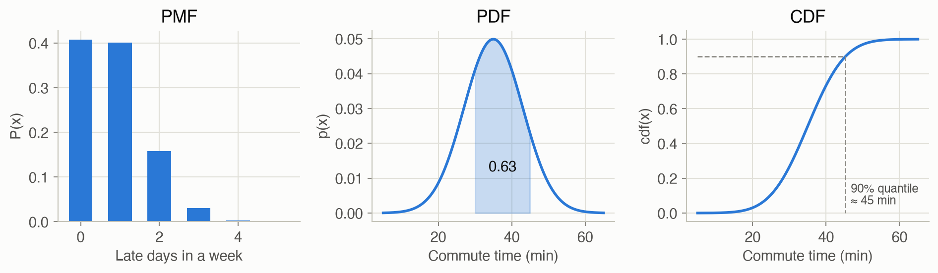
Probability is a degree of belief, and a distribution spreads it over the possible values. For a quantity with separate values, like “number of late days this week”, a probability mass function (PMF) gives each value a probability, and those add up to 1. For a continuous quantity, like “commute time in minutes”, a probability density function (PDF) is a curve, and probabilities are areas under it: the chance of a 30–45 minute trip is the area between 30 and 45. The Gaussian (bell curve) is the standard continuous shape. A mixture of several bell curves handles quantities with several typical values.
A joint distribution describes many variables together, and it explodes. To describe several variables at once, you need a probability for every combination of their values. Five yes/no variables have $2^5 = 32$ combinations; thirty have about a billion. Such a table can’t be stored, and there would never be enough data to fill it in.
Conditional distributions describe one variable given a few others. $P(x \mid y)$ is the probability of $x$ in the situations where $y$ holds. It is computed as $P(x, y) / P(y)$. For yes/no variables it’s a small table, a conditional probability table (CPT), such as “late 50% of the time if there’s a jam, 5% if not”. For continuous variables it’s a formula: a straight-line trend plus noise (linear Gaussian), or a smooth on/off switch (sigmoid).
A Bayesian network assembles conditionals into a full joint distribution. Draw a graph with an arrow from each variable to those it directly influences, with no loops. Give each variable one conditional table: its distribution given its parents (the variables pointing into it). Then the probability of any complete situation is the product of one entry from each table. This is the chain rule for Bayesian networks. The commute example needs 10 numbers instead of 31, and the savings grow exponentially with size.
The graph shows which variables can’t inform each other. Two variables are conditionally independent given some observations if learning one tells you nothing more about the other. You can read this off the graph with d-separation. Information flows along paths, a path through an observed middle variable is usually blocked, and one special case works the other way: two causes of a common effect become linked once the effect is observed. That effect is explaining away.

Vocabulary

Table 1: Terms used on this page.

Term	Plain meaning
Random variable	An uncertain quantity, like “was there a storm?” or “commute time”
PMF / PDF	Probability of each value (discrete) / density curve whose areas are probabilities (continuous)
CDF, quantile	Chance of at most $x$ / the value that is beaten a given fraction of the time
Joint distribution	Probabilities of every combination of values of several variables
Marginal	The distribution of some variables alone, found by summing the joint over the others
Conditional, CPT	Distribution of a variable given others; its table form for discrete variables
Parent / child	In a Bayesian network, a variable with an arrow into / out of another
Chain rule	The joint is the product of each variable’s conditional given its parents
Conditional independence	Once $Z$ is known, learning $Y$ tells you nothing more about $X$
d-separation	Reading conditional independence off the graph’s paths
Explaining away	Observing a common effect makes its independent causes compete

After this chapter you can

Describe an uncertain quantity with a PMF, PDF or mixture, and read probabilities as areas.
Count how many numbers a full joint table or a Bayesian network needs.
Build a small Bayesian network and compute the probability of any complete situation by the chain rule.
Tell from the graph alone whether two variables can inform each other, given what’s observed.

Intuition

Analogy

Imagine describing every possible morning before work. You track five yes/no facts: was there a storm, roadwork, a traffic jam, were you late, and did the radio warn of a storm? Listing a probability for every combination takes $2^5 = 32$ numbers. With 30 facts it would take about a billion.

But you don’t think that way. You think in local stories: storms and roadwork cause jams; jams make you late; storms trigger radio alerts. Each story needs only a few numbers (“if there’s a jam, I’m late half the time”). Chain the stories together and you can still recover the probability of any full morning, from just 10 numbers.

That “chain the local stories” idea is a Bayesian network. Figure 2 draws the one used throughout this page.

Figure 2: The morning-commute Bayesian network. Each arrow points from a cause to an effect; each variable is yes/no, and each comes with a small table of probabilities given its parents.

Probabilities as areas

Say your commute time is spread like a bell curve centered at 35 minutes. What’s the chance a trip takes exactly 35.000 minutes? Essentially zero: there are infinitely many possible times. The sensible question is about a range. The chance of 30–45 minutes is the area under the curve between 30 and 45, about 0.63. So the curve’s height (the density) is not itself a probability, and for a narrow curve it can be bigger than 1. Only areas are probabilities. See Equation 1 and Figure 3.

Why a full table explodes

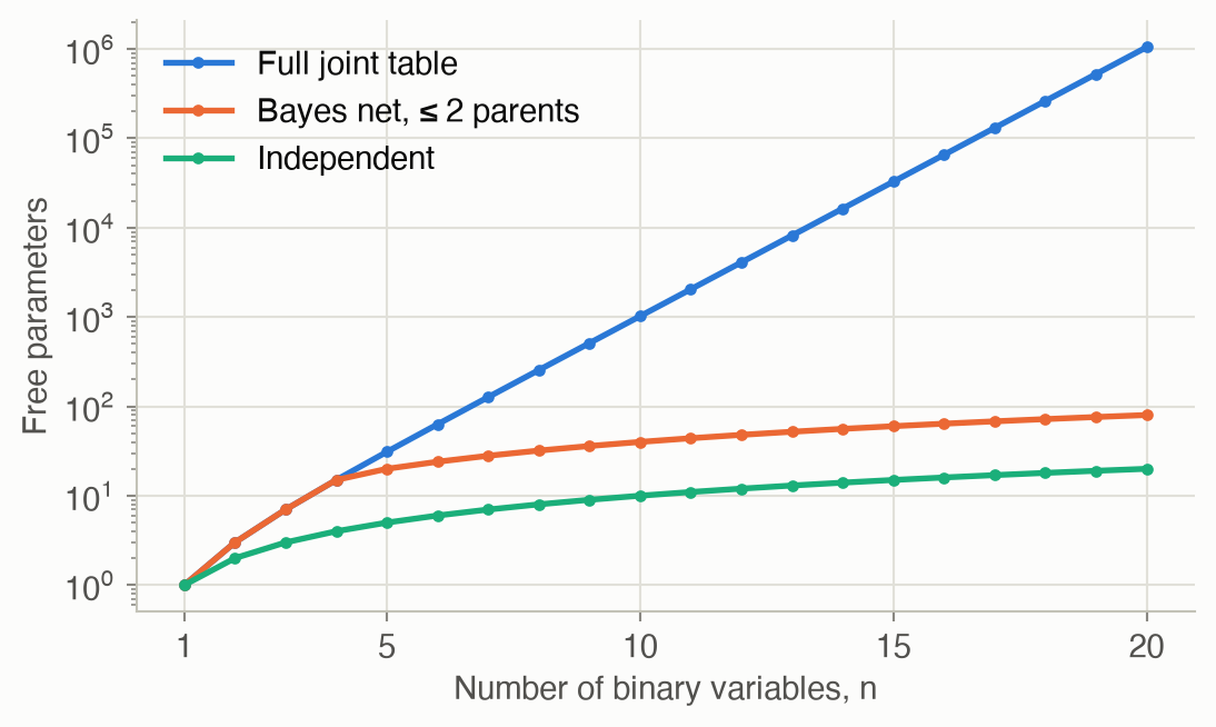
Five yes/no facts give 32 combinations, which is manageable. Each extra fact doubles the count: 10 facts give about a thousand, 20 about a million, 30 about a billion. Even if you could store a billion numbers, you could never observe enough mornings to estimate them. The fix is not a bigger table but a different representation. See Figure 6.

Conditionals as local stories

“If there’s a jam, I’m late half the time; if not, one time in twenty.” That is a conditional distribution: two numbers, $P(\text{late} \mid \text{jam}) = 0.5$ and $P(\text{late} \mid \text{no jam}) = 0.05$. It mentions only the jam, because once you know about the jam, the storm and the roadwork don’t change your lateness. Each variable’s story involves only its direct causes, which keeps every story small. See Equation 5.

Multiplying the stories together

How likely is this particular morning: a storm, no roadwork, a jam, late, and a radio alert? Walk through the stories in cause-before-effect order and multiply:

storm: 0.1;
no roadwork: 0.8;
a jam, given storm and no roadwork: 0.7;
late, given the jam: 0.5;
an alert, given the storm: 0.95.

The product is 0.027. Every complete morning’s probability comes out this way, so the ten numbers in the stories carry the same information as the 31 in a full table. That’s the chain rule, Equation 8.

Reading independence off the picture

Storms and roadwork have nothing to do with each other: learning there’s roadwork tells you nothing about the weather. But suppose you’re stuck in a jam. Now a storm is a plausible explanation (29% likely). If you then see roadwork, the jam is already explained, and a storm drops to 14%. The two causes became linked because you observed their common effect. The opposite happens on a chain: once you know whether there was a jam, the storm no longer tells you anything about being late. The graph shows which case you’re in. See Figure 7.

Formalism

Probability distributions (one variable)

A probability measures a degree of belief (ADM §2.1): 0 means certainly false, 1 means certainly true. A distribution assigns belief to every value a variable can take (ADM §2.2).

\[ \sum_{x} P(x) = 1 \quad\text{(discrete)} \qquad\qquad \int_{-\infty}^{\infty} p(x)\, dx = 1 \quad\text{(continuous)} \tag{1}\]

In words. For a discrete variable, the probabilities of all values add up to 1. For a continuous one, the density curve encloses an area of 1.

Term by term.

$P(x)$ is a probability mass function (PMF): the probability that the variable equals $x$ exactly.
$p(x)$ is a probability density function (PDF). It is not a probability, and it can exceed 1. Probabilities come from areas: $P(a \le x \le b) = \int_a^b p(x)\, dx$.
The distinction matters because a continuous variable takes any single exact value with probability 0.

The cumulative distribution function $\operatorname{cdf}(x) = P(X \le x)$ answers “what’s the chance of at most $x$?”. Its inverse, the quantile function, answers “what value is exceeded only $1 - \alpha$ of the time?”. For example, the 90% quantile of your commute time is the time you beat 9 days out of 10.

The most important continuous distribution:

\[ \mathcal{N}(x \mid \mu, \sigma^2) = \frac{1}{\sigma\sqrt{2\pi}} \exp\!\left(-\frac{(x - \mu)^2}{2\sigma^2}\right) \tag{2}\]

In words. A symmetric bell curve centered at $\mu$, whose width is set by $\sigma$.

Term by term.

$\mu$ is the mean: the center and the most likely value.
$\sigma$ is the standard deviation. About 68% of the probability lies within $\mu \pm \sigma$, and about 95% within $\mu \pm 2\sigma$.
$\frac{(x-\mu)^2}{2\sigma^2}$ penalizes distance from the mean, measured in units of $\sigma$. The exponential turns that penalty into a density that falls off fast.
$\frac{1}{\sigma\sqrt{2\pi}}$ is just the constant that makes the area equal to 1 (Equation 1).

Two other workhorses are the uniform $\mathcal{U}(x \mid a, b)$, which is flat on $[a, b]$, and the mixture, for data with several distinct modes:

\[ p(x) = \sum_{i=1}^{n} \rho_i\, \mathcal{N}(x \mid \mu_i, \sigma_i^2), \qquad \rho_i \ge 0,\ \ \sum_i \rho_i = 1 \tag{3}\]

In words. Pick one of $n$ bell curves at random, with probability $\rho_i$ for curve $i$, then draw from it.

Term by term. $\rho_i$ is the mixture weight, or how common component $i$ is. The weights sum to 1, so the mixture still integrates to 1. Commute times are a natural example: normal days cluster around 30 minutes, jam days around 50. You can try it in the interactive below.

Figure 3 shows a PMF, a PDF and a CDF side by side.

Three panels. The left is a bar chart over 0 to 5 late days, tallest at 0 and 1 and near zero from 3 on. The middle is a bell curve centered at 35 minutes, with the region from 30 to 45 shaded. The right is an S-shaped curve rising from 0 to 1, with a dashed line at probability 0.9 meeting the curve at about 45 minutes. — Figure 3: Three ways to describe a distribution. Left: a PMF, the number of late days in a 5-day week. Middle: a PDF, commute time in minutes, where the shaded area is the probability of a 30–45 minute trip. Right: the CDF of the same commute time, with the 90% quantile marked.

Joint distributions (many variables)

A joint distribution $P(x_1, \ldots, x_n)$ gives the probability of every combination of values (ADM §2.3). For $n$ binary variables, a full table has $2^n$ entries, and $2^n - 1$ free parameters, because the last entry is fixed by the rest summing to 1. That exponential growth is the central problem this chapter solves (Figure 6).

For continuous variables, the standard joint distribution is the multivariate Gaussian:

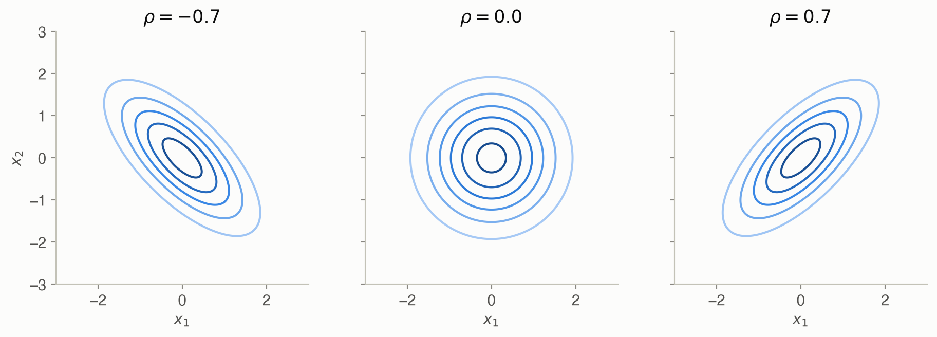
\[ \mathcal{N}(\mathbf{x} \mid \boldsymbol{\mu}, \boldsymbol{\Sigma}) = \frac{1}{(2\pi)^{n/2} |\boldsymbol{\Sigma}|^{1/2}} \exp\!\left(-\tfrac{1}{2} (\mathbf{x} - \boldsymbol{\mu})^\top \boldsymbol{\Sigma}^{-1} (\mathbf{x} - \boldsymbol{\mu})\right) \tag{4}\]

In words. A bell-shaped hill in $n$ dimensions. The mean $\boldsymbol{\mu}$ sets where the hill is; the covariance $\boldsymbol{\Sigma}$ sets its width in each direction and how the variables move together.

Term by term.

$\boldsymbol{\Sigma}_{ii}$ is the variance of variable $i$. $\boldsymbol{\Sigma}_{ij}$ is the covariance of $i$ and $j$: positive if they tend to rise together, negative if one tends to fall as the other rises.
$(\mathbf{x} - \boldsymbol{\mu})^\top \boldsymbol{\Sigma}^{-1} (\mathbf{x} - \boldsymbol{\mu})$ is a squared distance from the mean that accounts for the variables’ spreads and correlations (the Mahalanobis distance). The contours of equal density are ellipses.
$|\boldsymbol{\Sigma}|$, the determinant, measures the overall spread; it keeps the total volume equal to 1.
The joint needs only $n$ means and $n(n+1)/2$ covariances, far fewer than a table, because the Gaussian’s shape is fixed.

Three square contour plots of nested ellipses. With correlation minus 0.7 the ellipses tilt downward to the right; with correlation 0 they are circles; with correlation 0.7 they tilt upward to the right. — Figure 4: Density contours of a two-variable Gaussian with unit variances and three correlations. Correlation tilts and stretches the ellipses: with ρ = 0.7, a high x₁ makes a high x₂ likely.

Conditional distributions

The way out of the exponential table is to describe each variable given the few things it depends on (ADM §2.4).

\[ P(x \mid y) = \frac{P(x, y)}{P(y)} \tag{5}\]

In words. Among the situations where $y$ holds, what fraction also have $x$?

Term by term. $P(x, y)$ is how often $x$ and $y$ happen together. Dividing by $P(y)$ zooms in on the world where $y$ happened, and rescales it so that it sums to 1 again. Rearranged, $P(x, y) = P(x \mid y)\, P(y)$: a joint can be built from a conditional times a marginal. That identity is the seed of the Bayesian network.

A conditional probability table (CPT) stores $P(x \mid y)$ for discrete variables: one distribution over $x$ for each value of the parents $y$. Continuous variables need a formula instead. Two common ones:

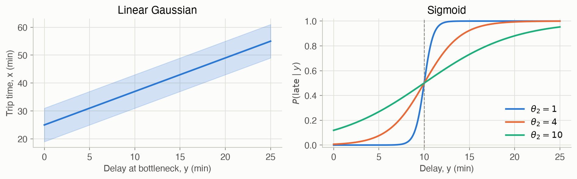
\[ p(x \mid y) = \mathcal{N}(x \mid m y + b,\ \sigma^2) \tag{6}\]

In words. $x$ is a straight-line function of $y$, plus bell-shaped noise.

Term by term. $m$ is the slope (how much $x$ moves per unit of $y$), $b$ is the intercept, and $\sigma$ is the noise around the line. For example, trip time might be $m = 1.2$ minutes per minute of delay, plus a baseline $b$, plus noise.

\[ P(x^1 \mid y) = \frac{1}{1 + \exp\!\left(-2\,\frac{y - \theta_1}{\theta_2}\right)} \tag{7}\]

In words. A smooth on/off switch. The probability that a binary $x$ is “yes” rises from 0 to 1 as a continuous $y$ passes a threshold.

Term by term.

$x^1$ means “$x$ takes value 1”, or yes. $x^0$ is no.
$\theta_1$ is the threshold: at $y = \theta_1$, the probability is exactly 0.5.
$\theta_2$ is the softness. A small $\theta_2$ gives an abrupt switch, and a large one a gradual ramp.

Two panels. The left shows a straight line rising from about 25 minutes at zero delay to about 55 at 25 minutes of delay, inside a shaded band of constant width. The right shows three S-shaped curves crossing 0.5 at a delay of 10 minutes: one steep, one moderate, one gradual. — Figure 5: Two conditional distributions for continuous parents. Left: a linear Gaussian, trip time given the delay at a bottleneck; the line is the mean and the band holds 95% of trips. Right: a sigmoid, the probability of being late given the delay, for three softness values θ₂ with threshold θ₁ = 10 minutes.

Bayesian networks

A Bayesian network is a directed acyclic graph with one node per variable, plus one conditional distribution per node given its parents (ADM §2.5). It encodes a joint distribution through one famous identity:

\[ P(x_{1:n}) = \prod_{i=1}^{n} P\big(x_i \mid \mathrm{pa}(x_i)\big) \tag{8}\]

In words. The probability of a complete situation is the product of each variable’s probability given its parents’ values in that situation.

Term by term.

$x_{1:n}$ is a full assignment: a value for every variable.
$\mathrm{pa}(x_i)$ is the values of $X_i$’s parents in the graph.
Each factor comes straight out of a small CPT.

Why it holds. The general chain rule, which comes from applying Equation 5 repeatedly, says $P(x_{1:n}) = \prod_i P(x_i \mid x_{1:i-1})$ for any ordering. Order the variables so that parents come before children. The network’s defining assumption is that each variable, given its parents, is independent of the other variables earlier in the order. So each factor shrinks to $P(x_i \mid \mathrm{pa}(x_i))$.

What it saves. A node with $k$ binary parents needs $2^k$ numbers, one $P(\text{yes})$ per parent combination. The commute network needs $1 + 1 + 4 + 2 + 2 = 10$ numbers, where the full table needs 31. With 20 variables and at most two parents each, the difference is at most 80 against about a million (Figure 6).

Line chart with the number of variables from 1 to 20 across and the number of parameters on a log scale up the side. The full-table line rises steeply and straight, reaching about a million at 20 variables. The Bayesian-network line rises gently to 80. The independent line is lowest, reaching 20. — Figure 6: Free parameters needed for n binary variables: a full joint table, a Bayesian network where each variable has at most 2 parents, and fully independent variables. The vertical axis is logarithmic, so the full table’s straight line is exponential growth.

Conditional independence

The graph also tells you, without any arithmetic, when learning one variable can’t change your belief about another (ADM §2.6).

\[ (X \perp Y \mid Z) \iff P(x, y \mid z) = P(x \mid z)\, P(y \mid z) \ \text{ for all } x, y, z \tag{9}\]

In words. Once you know $Z$, also learning $Y$ tells you nothing more about $X$.

Term by term. $\perp$ reads “is independent of”. The right side says the joint of $X$ and $Y$, given $Z$, splits into separate factors. Equivalently, $P(x \mid y, z) = P(x \mid z)$.

Whether a path between two variables carries information depends on the middle node of each three-node segment. There are three patterns, shown in Figure 7.

Figure 7: The three building blocks of d-separation. Observing the middle node (shaded) blocks a chain and a fork, but opens a collider.

Chain $S \to J \to L$: a storm makes a jam likelier, which makes being late likelier. If you already know whether there was a jam, the storm adds nothing about lateness. Observing the middle blocks.
Fork $A \leftarrow S \to J$: a radio alert and a jam share a cause. The alert suggests a storm, and so a jam. Once you know whether there was a storm, the alert adds nothing. Observing the middle blocks.
Collider $S \to J \leftarrow R$: storms and roadwork are unrelated, until you see a jam. Then learning there was roadwork explains away the jam and makes a storm less likely. Observing the middle, or any of its descendants, opens the path.

$X$ and $Y$ are d-separated by $Z$ if every path between them is blocked somewhere. d-separation guarantees $(X \perp Y \mid Z)$ for every choice of CPTs.

Worked example

The commute network’s tables, in code. (The network also has an entry in the problem gallery, where it can be loaded ready-made.)

from adm.bayes_net import BayesNet

def binary(p_yes):
    """CPT with last axis (no, yes), from P(yes) for each parent combination."""
    p_yes = np.asarray(p_yes, dtype=float)
    return np.stack([1 - p_yes, p_yes], axis=-1)

parents = {"S": (), "R": (), "J": ("S", "R"), "L": ("J",), "A": ("S",)}
commute = BayesNet(
    card={x: 2 for x in parents},
    parents=parents,
    cpt={
        "S": binary(0.1),                     # P(storm)
        "R": binary(0.2),                     # P(roadwork)
        "J": binary([[0.1, 0.6], [0.7, 0.9]]),  # P(jam | S, R); rows S, columns R
        "L": binary([0.05, 0.5]),             # P(late | J)
        "A": binary([0.02, 0.95]),            # P(alert | S)
    },
)

# Values are 1 = no, 2 = yes (Julia counts from 1).
struct BayesNet
    card; parents; cpt      # Dicts keyed by variable name (a Symbol)
end

# CPT with last axis (no, yes), from P(yes) for each parent combination.
binary(p_yes) = cat(1 .- p_yes, p_yes; dims = ndims(p_yes) + 1)

parents = Dict(:S => (), :R => (), :J => (:S, :R), :L => (:J,), :A => (:S,))
commute = BayesNet(
    Dict(x => 2 for x in keys(parents)),
    parents,
    Dict(:S => binary(0.1),                   # P(storm)
         :R => binary(0.2),                   # P(roadwork)
         :J => binary([0.1 0.6; 0.7 0.9]),    # P(jam | S, R); rows S, columns R
         :L => binary([0.05, 0.5]),           # P(late | J)
         :A => binary([0.02, 0.95])),         # P(alert | S)
)

A full morning, by the chain rule. What’s the probability of a storm, no roadwork, a jam, being late, and a radio alert? By Equation 8, multiply one entry from each table:

\[ P(s^1, r^0, j^1, l^1, a^1) = \underbrace{0.1}_{P(s^1)} \times \underbrace{0.8}_{P(r^0)} \times \underbrace{0.7}_{P(j^1 \mid s^1, r^0)} \times \underbrace{0.5}_{P(l^1 \mid j^1)} \times \underbrace{0.95}_{P(a^1 \mid s^1)} = 0.0266 \]

How often is there a jam? Sum over the four combinations of its parents:

\[ P(j^1) = \sum_{s, r} P(s)\, P(r)\, P(j^1 \mid s, r) = 0.9(0.8)(0.1) + 0.9(0.2)(0.6) + 0.1(0.8)(0.7) + 0.1(0.2)(0.9) = 0.254 \]

Then $P(l^1) = 0.254 \times 0.5 + 0.746 \times 0.05 = 0.164$: you’re late about one day in six. That number fed the PMF in Figure 3.

Explaining away, in numbers. You’re stuck in a jam. How likely is it that there was a storm?

\[ P(s^1 \mid j^1) = \frac{P(s^1, j^1)}{P(j^1)} = \frac{0.1\,(0.8 \times 0.7 + 0.2 \times 0.9)}{0.254} = \frac{0.074}{0.254} \approx 0.29 \]

Now you also see roadwork. The roadwork alone would explain the jam, so a storm becomes less likely:

\[ P(s^1 \mid j^1, r^1) = \frac{0.1 \times 0.9}{0.1 \times 0.9 + 0.9 \times 0.6} = \frac{0.09}{0.63} \approx 0.14 \]

Storm and roadwork are independent a priori, but dependent once the jam is known. That is the collider pattern at work. Table 2 confirms these numbers from the full joint table.

Table 2: The worked example’s numbers, computed from the full 32-entry joint table built by the chain rule.

Quantity	Value
P(s¹, r⁰, j¹, l¹, a¹)	0.0266
P(j¹)	0.2540
P(l¹)	0.1643
P(s¹ \| j¹)	0.2913
P(s¹ \| j¹, r¹)	0.1429
Parameters: network vs full table	10 vs 31

Interactive

Explore independence in the commute network

Pick two variables and any set of observed ones. The explorer reports whether the two are independent, and if not, it highlights an active trail that carries information between them. Observed variables are shaded, as in Figure 7. Try Storm vs. Roadwork with nothing observed, then observe Late.

dsep = FileAttachment("data/ch02-dsep.json").json()
names = Object.fromEntries(dsep.nodes.map(d => [d.id, d.name]))
viewof x = Inputs.select(dsep.nodes.map(d => d.id), {label: "Is", value: "S", format: v => names[v]})
viewof y = Inputs.select(dsep.nodes.map(d => d.id), {label: "independent of", value: "R", format: v => names[v]})
viewof given = Inputs.checkbox(dsep.nodes.map(d => d.id).filter(v => v !== x && v !== y),
                               {label: "given (observed)", format: v => names[v]})

trail = x === y ? undefined : dsep.queries[[x, y, [...given].sort().join(",")].join("|")]
md`${x === y ? "Pick two different variables." : trail === null
  ? `**Yes: ${names[x]} ⊥ ${names[y]}${given.length ? " | " + given.map(v => names[v]).join(", ") : ""}.** Every path between them is blocked.`
  : `**No: they are dependent.** Active trail: ${trail.map(v => names[v]).join(" — ")}.`}`

{
  const W = 420, H = 320, hw = 62, hh = 18, s = dsep.style;
  const pos = Object.fromEntries(dsep.nodes.map(d => [d.id, d]));
  const hot = new Set((trail || []).slice(1).map((v, i) => [trail[i], v].sort().join("")));
  const svg = d3.create("svg").attr("viewBox", [0, 0, W, H]).attr("width", W)
    .style("background", s.surface).style("font", "13px system-ui, sans-serif");
  for (const [id, c] of [["arrow", s.muted], ["arrow-hot", s.orange]])
    svg.append("defs").append("marker").attr("id", id).attr("viewBox", "0 0 10 10").attr("refX", 10).attr("refY", 5)
      .attr("markerWidth", 7).attr("markerHeight", 7).attr("orient", "auto")
      .append("path").attr("d", "M0,0L10,5L0,10z").attr("fill", c);
  const edgePoint = (a, b) => {           // where the line from a to b leaves a's box
    const dx = b.x - a.x, dy = b.y - a.y, k = 1 / Math.max(Math.abs(dx) / hw, Math.abs(dy) / hh);
    return [a.x + k * dx, a.y + k * dy];
  };
  for (const [u, v] of dsep.edges) {
    const on = hot.has([u, v].sort().join(""));
    const [x1, y1] = edgePoint(pos[u], pos[v]), [x2, y2] = edgePoint(pos[v], pos[u]);
    svg.append("line").attr("x1", x1).attr("y1", y1).attr("x2", x2).attr("y2", y2)
      .attr("stroke", on ? s.orange : s.muted).attr("stroke-width", on ? 4 : 1.5)
      .attr("marker-end", `url(#${on ? "arrow-hot" : "arrow"})`);
  }
  for (const d of dsep.nodes) {
    const g = svg.append("g").attr("transform", `translate(${d.x - hw},${d.y - hh})`);
    g.append("rect").attr("width", 2 * hw).attr("height", 2 * hh).attr("rx", 8)
      .attr("fill", given.includes(d.id) ? s.observed : (d.id === x || d.id === y) ? s.blueFill : "white")
      .attr("stroke", (d.id === x || d.id === y) ? s.blue : s.muted).attr("stroke-width", (d.id === x || d.id === y) ? 2.5 : 1.2);
    g.append("text").attr("x", hw).attr("y", hh + 5).attr("text-anchor", "middle").attr("fill", s.ink).text(d.name);
  }
  return svg.node();
}

Figure 8: d-separation explorer for the commute network. The orange edges form an active trail, if there is one.

Mix two commute-time distributions

Commute time is a mixture (Equation 3) of normal days, $\mathcal{N}(30, 4^2)$, and jam days, $\mathcal{N}(50, 8^2)$. The slider sets the weight on jam days. It starts at the network’s value, $P(j^1) = 0.254$.

Figure 9: A two-component Gaussian mixture of commute times. Dashed curves are the weighted components; the solid curve is their sum. Use the slider to change the weight on jam days.

Algorithms & code

Chain rule, joint table, and parameter count

These implement Equation 8. joint_table applies it to every assignment, which is fine for 5 variables and hopeless for 50. Chapter 3 is about avoiding exactly that.

def probability(bn: BayesNet, assignment: dict) -> float:
    """P(assignment) by the chain rule: one CPT entry per variable."""
    p = 1.0
    for x, pa in bn.parents.items():
        # CPT axes are (parents..., x), so index with the parents' values
        # first and x's own value last.
        index = tuple(assignment[q] for q in pa) + (assignment[x],)
        p *= bn.cpt[x][index]
    return p

def joint_table(bn: BayesNet) -> np.ndarray:
    """The full joint distribution as an array, axes in `bn.parents` order."""
    names = list(bn.parents)
    table = np.zeros([bn.card[x] for x in names])
    for values in product(*(range(bn.card[x]) for x in names)):
        table[values] = probability(bn, dict(zip(names, values)))
    return table

def num_parameters(bn: BayesNet) -> int:
    """Independent numbers in all the CPTs (each row loses one: it sums to 1)."""
    return sum(
        prod(bn.card[q] for q in pa) * (bn.card[x] - 1)
        for x, pa in bn.parents.items()
    )

# P(assignment) by the chain rule: one CPT entry per variable.
# `...` splats the parents' values into separate indices; x's own value comes last.
probability(bn, a) = prod(bn.cpt[x][(a[q] for q in pa)..., a[x]] for (x, pa) in bn.parents)

# The full joint distribution as an array, with axes in the given order.
function joint_table(bn, order)
    table = zeros(Tuple(bn.card[x] for x in order))
    for idx in CartesianIndices(table)
        table[idx] = probability(bn, Dict(zip(order, Tuple(idx))))
    end
    return table
end

# Independent numbers in all the CPTs (each row loses one: it sums to 1).
num_parameters(bn) = sum(prod((bn.card[q] for q in pa); init = 1) * (bn.card[x] - 1)
                         for (x, pa) in bn.parents)

d-separation by searching for an active trail

The search walks the graph from $X$, keeping track of whether it arrived at each node from a child (“up”) or from a parent (“down”). That direction is what decides whether a node is a chain, fork or collider on the current path. If it ever reaches $Y$, the path it followed is an active trail.

def active_trail(parents: dict, x: str, y: str, given=()) -> list | None:
    """An active trail from x to y given the observed set, or None if none.

    Searches (node, direction) pairs: "up" means we arrived from a child,
    "down" means we arrived from a parent. A trail through a node is blocked
    if the node is observed, except at a v-structure (collider), which is
    active only if the collider or one of its descendants is observed.
    """
    given = set(given)
    children = {v: [c for c in parents if v in parents[c]] for v in parents}
    # A collider is active if it or a descendant is observed, i.e. if it is
    # an ancestor of (or in) the observed set.
    active_colliders, frontier = set(), list(given)
    while frontier:
        v = frontier.pop()
        if v not in active_colliders:
            active_colliders.add(v)
            frontier.extend(parents[v])
    came_from = {(x, "up"): None}
    queue = [(x, "up")]
    while queue:
        node, direction = state = queue.pop(0)
        if node == y and node not in given:
            trail = []
            while state is not None:
                trail.append(state[0])
                state = came_from[state]
            return trail[::-1]
        moves = []
        if direction == "up" and node not in given:
            moves += [(p, "up") for p in parents[node]]
            moves += [(c, "down") for c in children[node]]
        elif direction == "down":
            if node not in given:
                moves += [(c, "down") for c in children[node]]
            if node in active_colliders:
                moves += [(p, "up") for p in parents[node]]
        for move in moves:
            if move not in came_from:
                came_from[move] = state
                queue.append(move)
    return None

def d_separated(parents: dict, x: str, y: str, given=()) -> bool:
    """True if x and y are conditionally independent given `given`."""
    return active_trail(parents, x, y, given) is None

function active_trail(parents, x, y, given = ())
    given = Set(given)
    children = Dict(v => [c for c in keys(parents) if v in parents[c]] for v in keys(parents))
    # A collider is active if it or a descendant is observed.
    active_colliders, frontier = Set{Symbol}(), collect(given)
    while !isempty(frontier)
        v = pop!(frontier)
        v in active_colliders && continue
        push!(active_colliders, v)
        append!(frontier, parents[v])
    end
    came_from = Dict{Tuple{Symbol, Symbol}, Any}((x, :up) => nothing)
    queue = [(x, :up)]
    while !isempty(queue)
        state = popfirst!(queue)
        node, direction = state
        if node == y && !(node in given)
            trail = Symbol[]
            while state !== nothing
                push!(trail, state[1])
                state = came_from[state]
            end
            return reverse(trail)
        end
        moves = Tuple{Symbol, Symbol}[]
        if direction == :up && !(node in given)
            append!(moves, [(p, :up) for p in parents[node]], [(c, :down) for c in children[node]])
        elseif direction == :down
            node in given || append!(moves, [(c, :down) for c in children[node]])
            node in active_colliders && append!(moves, [(p, :up) for p in parents[node]])
        end
        for m in moves
            haskey(came_from, m) || (came_from[m] = state; push!(queue, m))
        end
    end
    return nothing
end

d_separated(parents, x, y, given = ()) = active_trail(parents, x, y, given) === nothing

Run them on the commute network

p_morning = probability(commute, {"S": 1, "R": 0, "J": 1, "L": 1, "A": 1})
n_params = num_parameters(commute)
storm_roadwork = d_separated(parents, "S", "R")
storm_roadwork_given_late = d_separated(parents, "S", "R", ["L"])
trail = active_trail(parents, "A", "L")

p_morning = probability(commute, Dict(:S => 2, :R => 1, :J => 2, :L => 2, :A => 2))
@assert p_morning ≈ 0.1 * 0.8 * 0.7 * 0.5 * 0.95
@assert num_parameters(commute) == 10
joint = joint_table(commute, [:S, :R, :J, :L, :A])
@assert sum(joint) ≈ 1 && sum(joint[:, :, :, 2, :]) ≈ 0.1643
@assert d_separated(parents, :S, :R) && !d_separated(parents, :S, :R, (:L,))
@assert active_trail(parents, :A, :L) == [:A, :S, :J, :L]

P(storm, no roadwork, jam, late, alert) = 0.0266
Parameters: 10 in the network vs 31 in a full table
Storm ⊥ Roadwork: True;  Storm ⊥ Roadwork | Late: False
Active trail from Radio alert to Late: A → S → J → L

Reading the Julia code (for Python programmers)

Symbols like :S are lightweight names, a common choice for dictionary keys. They’re like interned strings.
cat(a, b; dims = k) stacks arrays along a new axis k, like np.stack([a, b], axis=-1) here.
Splatting: bn.cpt[x][(a[q] for q in pa)..., a[x]] expands the parents’ values into separate indices, like table[(*parent_values, x_value)] in Python.
CartesianIndices(table) loops over every index tuple of an array, like itertools.product(*map(range, table.shape)).
prod(...; init = 1) gives 1 for an empty product, which is needed for a node with no parents. Python’s math.prod does that automatically.

Solved problems

Problem 1: counting parameters. A network has six binary variables. $A$ and $B$ have no parents; $C$ has parents $A, B$; $D$ has parent $C$; $E$ has parents $C, D$; $F$ has parents $B, E$. How many free parameters does it need, and how many would a full joint table need?

Solution

Each binary node needs $2^{k}$ numbers, where $k$ is its number of parents: $A$: 1, $B$: 1, $C$: 4, $D$: 2, $E$: 4, $F$: 4. The total is 16. A full table needs $2^6 - 1 = $ 63.

Problem 2: reading independence off the graph. In the commute network, decide each of the following, and name the blocking or active pattern: (a) $A \perp R$; (b) $A \perp R \mid J$; (c) $A \perp L \mid S$; (d) $S \perp R \mid L$.

Solution

Independent. The only path is $A \leftarrow S \to J \leftarrow R$, and the collider $J$ is unobserved (as is its descendant $L$), so it blocks.
Dependent. Observing $J$ opens the collider. The fork at $S$ is unobserved, so it passes, and the trail $A - S - J - R$ is active.
Independent. The path $A \leftarrow S \to J \to L$ has a fork at $S$, which is observed and so blocks.
Dependent. $L$ is a descendant of the collider $J$. Observing it opens $S \to J \leftarrow R$. Intuitively, being late suggests a jam, which then needs an explanation.

Check them all in the explorer above.

Problem 3: a Gaussian probability. Commute time is $\mathcal{N}(35, 8^2)$ minutes. Using the rule of thumb that about 95% of the probability lies within $2\sigma$ of the mean, what range covers 95% of commutes? About what fraction of commutes take longer than 51 minutes?

Solution

$35 \pm 2 \times 8$ gives 19 to 51 minutes. The remaining 5% is split evenly between the two tails, so about 2.5% of commutes take longer than 51 minutes. (The exact value is 2.3%.)

Problem 4: explaining away, from scratch. Change the commute network so that roadwork is common, $P(r^1) = 0.5$, and keep everything else. Compute $P(s^1 \mid j^1)$. Is it higher or lower than the original 0.29, and why?

Solution

$P(s^1, j^1) = 0.1\,(0.5 \times 0.7 + 0.5 \times 0.9) = 0.08$, and $P(s^0, j^1) = 0.9\,(0.5 \times 0.1 + 0.5 \times 0.6) = 0.315$. So $P(s^1 \mid j^1) = 0.08 / 0.395 \approx$ 0.20, which is lower than 0.29. With roadwork common, a jam is more easily explained without a storm, so seeing a jam is weaker evidence for one. This is explaining away again, now working through the prior on the competing cause.

Recap

Distributions describe belief about one quantity: a PMF for discrete values, a PDF for continuous ones, with probabilities as areas (Equation 1). The Gaussian (Equation 2) and mixtures (Equation 3) are the everyday building blocks. Why it matters: every model later in the book, whether transitions, observations or rewards, is built from these pieces.
Joint distributions over many variables grow exponentially: $2^n - 1$ numbers for $n$ binary variables. Why it matters: this is the core obstacle to reasoning about realistic systems, and every representation afterward is a way around it.
Conditional distributions describe one variable given a few others: tables, linear Gaussians (Equation 6), sigmoids (Equation 7). Why it matters: they are the “local stories” that stay small, and they reappear as transition models $T(s' \mid s, a)$ in Ch 7 and observation models $O(o \mid a, s')$ in Ch 19.
A Bayesian network multiplies those local stories into a full joint (Equation 8), with far fewer parameters. Why it matters: it is the representation that Ch 3 (inference), Ch 4 (learning parameters) and Ch 5 (learning structure) all work on, and decision networks in Ch 6 extend it.
The graph reveals independence through d-separation: chains and forks are blocked by observing the middle; colliders are opened by it. Why it matters: independence is what makes inference and learning tractable, and explaining away is a real, often counterintuitive effect in diagnosis.

Cheat sheet & connections

Table 3: Key equations from this page (★ = well-known by name).

Name	Formula	Ref
Normalization	$\sum_x P(x) = 1$, $\ \int p(x)\,dx = 1$	Equation 1
★ Gaussian	$\mathcal{N}(x \mid \mu, \sigma^2) = \frac{1}{\sigma\sqrt{2\pi}} e^{-(x-\mu)^2 / 2\sigma^2}$	Equation 2
Mixture	$p(x) = \sum_i \rho_i \mathcal{N}(x \mid \mu_i, \sigma_i^2)$	Equation 3
★ Multivariate Gaussian	$\mathcal{N}(\mathbf{x} \mid \boldsymbol\mu, \boldsymbol\Sigma)$, with elliptical contours	Equation 4
★ Conditional probability	$P(x \mid y) = P(x, y) / P(y)$	Equation 5
Linear Gaussian	$p(x \mid y) = \mathcal{N}(x \mid my + b, \sigma^2)$	Equation 6
Sigmoid	$P(x^1 \mid y) = 1 / (1 + e^{-2(y - \theta_1)/\theta_2})$	Equation 7
★ Chain rule (Bayes net)	$P(x_{1:n}) = \prod_i P(x_i \mid \mathrm{pa}(x_i))$	Equation 8
Conditional independence	$P(x, y \mid z) = P(x \mid z) P(y \mid z)$	Equation 9

d-separation in one line: a path is blocked if it has an observed chain or fork node, or an unobserved collider with no observed descendants.

Common pitfalls

Treating a density as a probability. $p(x) = 2$ is fine for a narrow distribution; only areas are probabilities.
Forgetting that CPT rows sum to 1. Store $P(\text{yes})$ and derive $P(\text{no})$, or check each row.
Reading arrows as proof of causation. A Bayesian network only encodes independence. Arrows drawn from cause to effect make the tables small and easy to fill in, but the math doesn’t require it.
Assuming observed evidence can only reduce dependence. Observing a collider or one of its descendants creates dependence (explaining away).

Connections

Ch 3 · Inference computes queries like $P(s^1 \mid j^1)$ without building the full joint table.
Ch 4 · Parameter Learning estimates the CPT numbers from data.
Ch 5 · Structure Learning learns the graph itself.
Ch 6 · Simple Decisions adds decision and utility nodes to make decision networks.
Ch 19 · Beliefs uses the same conditional-distribution building blocks for dynamics and sensors.
Appendix B · Probability Distributions: the uniform, Gaussian, Beta and Dirichlet families, with plots.