Week 1 · Introduction to Robot Learning
Lecture of 16 February 2026
Big picture
Where this week fits
This is the start. The lecture sets out why robotics is hard in a way that language and vision are not, what “robot learning” means, and why the field now seems close to the kind of shift that large models brought to language ▶ 07:08. The rest of the course splits in two: the fundamentals (Weeks 2–5), then scaling robot learning to large models and data (Weeks 6–11).
How the course runs. Each Monday has a lecture of about 45 minutes, then student-led discussions of the week’s papers, in which one group presents a paper and another plays the critical reviewer, and on most weeks a short talk by a guest researcher ▶ 08:21 ▶ 10:26. Thursdays are TA sessions on the homework. The first half has four individual homeworks; the second half is group projects on real robots, a fleet of SO-101 arms with a leader–follower (“puppeteering”) setup for collecting demonstrations ▶ 13:01 ▶ 18:51. This site follows the lectures, papers and guest talks; it does not cover the homework or the projects.
The question this week answers: why can’t we simply program robots to work in our homes, and what does learning from data change?
The key ideas at a glance
- Classic robots sense, plan, then act. Shakey (1966) looked at its world, planned a path, and executed it. Factory robots still work this way, and it works as long as the world is structured and the robot knows exactly where everything is.
- Planning breaks when sensing is imperfect. Small errors in the robot’s estimate of the world, or in its motors, add up when the plan is executed blind. Closing the loop, re-sensing and re-deciding at every step, is the first defence, and the policies of this course work that way.
- Moravec’s paradox. Abstract reasoning is easy for computers; the physical skills a toddler has are hard. There is no internet-sized data set of how to grasp a mug.
- Robot learning = robotics + machine learning. Instead of hand-coding behaviour, a robot acquires skills from data and experience.
- The hardware has been ready for a while; the brain is missing. A 2007 robot tidying a room was teleoperated. What has changed since: compute, data at scale, and large models.
- Robotics as multimodal sequence modeling. Treat camera images, language instructions and robot actions all as tokens, and train one large model to continue the sequence with the right action tokens.
- But robots are not chatbots. Robot data is scarce and varied, control must be fast, and testing on hardware is slow and expensive.
- Two families of algorithms. Imitation learning copies demonstrations, much like supervised learning; reinforcement learning learns by trial and error from a reward. Either way, the robot’s actions change what it sees next, so its data are not independent samples.
Vocabulary
| Term | Plain meaning |
|---|---|
| Sense-plan-act | Perceive the world, compute a complete plan, then execute it |
| State estimation | Working out where the robot and everything around it are, from sensor data |
| Open loop | Executing actions without checking the result along the way |
| Closed loop | Choosing each action from the latest observation |
| Policy | A rule that picks the robot’s next action from what it observes |
| Robot learning | Getting a robot’s behaviour from data and experience instead of hand-written rules |
| Generalist policy | One policy for many tasks, robots and environments |
| Token | A discrete symbol a sequence model reads and writes: a word piece, an image patch, or a binned action |
| Vision-language-action model (VLA) | A vision-language model fine-tuned to output robot actions as tokens |
| i.i.d. | Independent and identically distributed: each data point drawn separately from the same distribution |
After this week you can
- Explain why sense-plan-act robots need near-perfect state estimation, and why closing the loop helps.
- State Moravec’s paradox and what it implies for robot data.
- Describe how a model like RT-2 turns continuous robot actions into tokens, and what that costs in precision.
- Say how imitation learning and reinforcement learning differ, and why neither has i.i.d. data.
A tour of the course
| Week | Lecture | In one line |
|---|---|---|
| 1 | Introduction | Why robot learning, and why now (this page) |
| 2 | Robot Control & MDPs | The mathematical language of robot–environment interaction |
| 3 | Imitation Learning | Learning a policy from expert demonstrations, and why copying drifts |
| 4–5 | Reinforcement Learning I and II | Learning from reward by trial and error, online and offline |
| 6 | Generative Models | Policies that output whole distributions of actions |
| 7 | Sequence Modeling and Transformers | The architectures behind language models, applied to actions |
| 8 | World Models | Models that predict how the world will respond |
| 9 | Generalist Robot Policies | One policy for many tasks and robots |
| 10 | Embodied Reasoning and Test-time Scaling | High-level reasoning for robots |
| 11 | Frontiers & Open Problems | What is still unsolved |
| 12 | Guest Lectures | Talks from the field, and the course reviewed in one table |
The lecturer describes the second half as the architectures of the foundation-model era: generative models, sequence models and transformers, world models and high-level reasoning ▶ 58:24.
Intuition
TipAnalogy
Walking to a door across a dark room, you can memorize the route with the lights on and then walk it blind, or keep a hand on the wall and correct as you go. Memorizing works if your picture of the room was exact and your steps are precise. A few degrees off at the start, or a short step halfway, and you meet the wall. Classic robots memorize the route; learned policies keep a hand on the wall.
Why build robots at all
The lecture’s answer is practical: jobs that are dangerous, distant or demanding (space, the deep sea, mines, disaster sites), health care, and care for ageing societies ▶ 24:27.
Sense, plan, act
Shakey, built at SRI in the 1960s, looked at its world through a camera, planned with search algorithms (the lecture notes that A* was developed for it), and pushed boxes around rooms ▶ 26:43. That sense-plan-act loop, run once per decision, is still how most industrial robots work: sense, plan a geometric path in a known map, execute with high precision ▶ 28:58. It works superbly in structured settings such as a car assembly line, because there the robot’s picture of the world is right ▶ 30:25.
The first toy on this page shows the difference. A robot starts on the left of a room and must pass a doorway in a wall to reach a goal on the right. The sense-plan-act robot estimates its starting position once, with error σ, plans a path through the door, and walks it. The closed-loop robot gets an equally noisy estimate at every step and heads for its next waypoint from there. Both robots’ motors land each step a little off (a standard deviation of 0.02 per step).
What to watch for. The orange robots set off together, but each follows a plan made from a slightly wrong starting point, so the bundle fans out as it walks. By the end, 6 of 12 sit in the circle, 1 has hit the wall beside the doorway, and the rest stop short or wide of the goal. The blue robots wobble more step to step, because each new estimate is noisy, but the wobbles don’t add up: every step aims at the next waypoint from wherever the robot now thinks it is, and all 12 arrive.
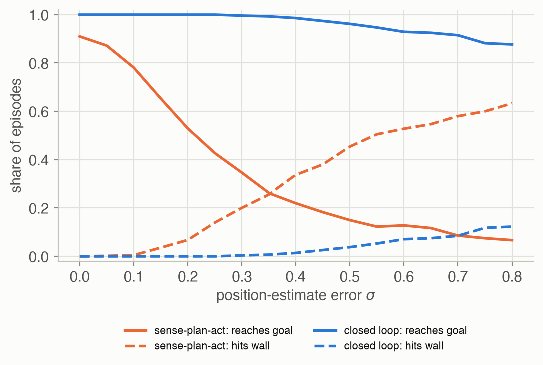
With a perfect estimate (σ = 0) the closed-loop robot always arrives; the sense-plan-act robot arrives in only 91% of episodes, because its small motor errors add up over the whole walk and nothing corrects them. As σ grows, sense-plan-act success falls below half at σ ≈ 0.21, and at σ = 0.8 63% of its runs end in the wall. The closed-loop robot succeeds every time up to σ = 0.25 and still 88% of the time at σ = 0.8, because each step’s error is independent and gets corrected at the next step.
When state estimation fails
The lecture’s videos make the same point with real hardware. Humanoids at the 2015 DARPA Robotics Challenge fell over opening doors and turning valves; later Atlas demonstrations relied on markers placed around the room so the robot always knew exactly where it was, and a few centimetres of error could end in a fall ▶ 31:43. Even the best engineered robots have depended on near-perfect state estimation.
Moravec’s paradox
Hans Moravec observed in 1988 that what humans find hard, such as chess and mathematics, is relatively easy for computers, while what a toddler does without thinking, picking up a cup, is very hard ▶ 33:28. One reason the lecture gives: there is no internet of grasping. The lecturer’s own PhD-era robot, grasping a mug from point clouds with an analytical grasp planner, crushed it.
What robot learning is, and what counts as a robot
The course defines robot learning as solving robotics with machine learning: perception and control on one side, imitation, reinforcement and representation learning on the other, and data-driven methods filling the gaps that hand-built models leave ▶ 35:56. Is a dishwasher a robot? A teleoperated surgical robot? ChatGPT on a phone? The class discussion landed on two tests: does it change the physical world, and does it act autonomously ▶ 38:09. Robot learning wants all three qualities at once: an appliance’s reliability, a surgical arm’s dexterity, and a foundation model’s general reasoning.
Why we don’t have home robots yet
In 2007 a Stanford robot, the PR1, was filmed tidying a room. It was teleoperated ▶ 40:58. The hardware to do housework has existed for almost two decades; the missing piece is the software, the brain that makes it autonomous. Since then three things have changed: capable humanoid hardware from several companies, far more compute, and data at a scale that would take a person tens of thousands of years to read ▶ 44:01 (see the worked example).
Generalist policies and actions as tokens
The lecture’s “north star” is a generalist robot policy: one model that takes a large, diverse robot data set and outputs actions for any task, on any robot, in any environment ▶ 47:20. The Open X-Embodiment collaboration pooled data from 22 robot types to make that possible ▶ 48:53.
The trick that connects this to large language models: a robot policy that maps “image + instruction” to “action” looks like a vision-language model that maps “image + question” to “answer”, if the actions are written as tokens ▶ 52:04.
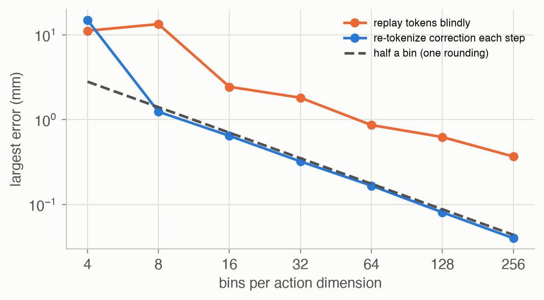
How do you write a continuous action as a token? RT-2 cuts each action dimension into 256 equal bins and writes the bin’s number (Equation 4). That loses a little precision every step. The second toy replays a 0.6 m reaching motion through tokens. Replayed blind, the rounding errors add up; a robot that re-observes where it is and tokenizes the correction keeps the error to one rounding. With 256 bins the largest deviation from the demonstrated path is 0.37 mm replayed blind and 0.04 mm closed loop; with 16 bins, 2.4 mm and 0.6 mm.
Not quite: why robots aren’t chatbots
“So we train a large transformer on robot data and we’re done?” Not quite ▶ 52:36. Robot data is scarce, because a person usually has to teleoperate or supervise every minute of it. It is multimodal and heterogeneous, since every robot has different sensors and actuators. The model must run in real time on the robot, so a giant model behind a slow API won’t do ▶ 53:59. And evaluating a policy on real hardware is slow, expensive and hard to reproduce ▶ 54:27.
Two families of algorithms
Most of the course builds on two frameworks ▶ 54:45. Imitation learning is close to supervised learning: learn a function from observations to the expert’s actions. Reinforcement learning learns a policy by trial and error to maximize a reward. In both, the robot’s own actions change what it observes next, so its data are not independent samples (Equation 2), which breaks a basic assumption of supervised learning ▶ 56:28. Week 3 shows what that costs.
One shift, three fields
The lecture ends by showing the same change in three places ▶ 59:59. Housework: from the teleoperated PR1 of 2007 to recent videos of robots doing similar tidying tasks autonomously. Driving: from the 2005 DARPA challenge, where vehicles with stacks of sensors and probabilistic models struggled across the desert, to cars that now drive themselves to their buyers ▶ 1:01:00. Humanoids: from the 2015 DARPA Robotics Challenge, where the best machines struggled to open a door or walk straight, to the smooth, dexterous humanoid demonstrations of today ▶ 1:01:30. In each case the move is from hand-coded behaviour to learned behaviour, and the course is about the machinery behind that move. (These are the lecturer’s examples; the demos are companies’ own videos, with the caveats about demos that Week 11 spells out.)
Why study it? The lecturer gave three reasons ▶ 1:03:03: the field spans the whole stack, from reasoning in foundation models down to the PID controllers that move the motors; its algorithms carry over across robots, from cars to humanoids to planetary rovers; and it may be close to its own “ChatGPT moment”.
Key concepts & formulae
Supervised learning assumes independent examples
\[ \begin{aligned} \theta^\star &= \arg\min_\theta \; \frac{1}{N}\sum_{i=1}^{N} \ell\big(f_\theta(x_i),\, y_i\big) \\ (x_i, y_i) &\overset{\text{i.i.d.}}{\sim} p(x, y) \end{aligned} \tag{1}\]
In words. Fit a function so that its predictions match the labels on the training examples, where every example is drawn on its own from one fixed distribution.
Term by term.
- \(f_\theta\): the model, with parameters \(\theta\); \(x_i\) an input, \(y_i\) its label.
- \(\ell\): a loss that is small when the prediction matches the label, such as squared error.
- i.i.d.: drawing \((x_1, y_1)\) tells you nothing about \((x_2, y_2)\), and test inputs come from the same \(p\) as training inputs. Classifying one cat photo does not change the next photo.
The robot loop breaks that assumption
\[ \begin{aligned} a_t &\sim \pi(a_t \mid o_t) \\ s_{t+1} &\sim p(s_{t+1} \mid s_t, a_t) \\ o_{t+1} &\sim p(o_{t+1} \mid s_{t+1}) \end{aligned} \tag{2}\]
In words. The robot picks an action from what it observes, the world moves to a new state that depends on that action, and the robot observes the new state.
Term by term.
- \(\pi\): the policy, the thing robot learning produces.
- \(s_t\): the true state of the world; \(o_t\): what the robot’s sensors report about it. They differ, which is exactly the state-estimation problem.
- \(p(s_{t+1} \mid s_t, a_t)\): the dynamics. Because \(a_t\) appears here, the next observation depends on the robot’s own choice: consecutive data points are not independent, and a different policy sees a different distribution of states. Week 2 builds this into Markov decision processes.
Open loop and closed loop
\[ \begin{aligned} \text{open loop:}\quad a_t &= \text{plan}_t(\hat{s}_0) \\ \text{closed loop:}\quad a_t &= \pi(\hat{s}_t) \end{aligned} \tag{3}\]
In words. An open-loop controller fixes every action in advance from one estimate of the start; a closed-loop controller computes each action from the latest estimate.
Term by term.
- \(\hat{s}_0\), \(\hat{s}_t\): the robot’s estimates of its state at the start and at step \(t\), never exactly right.
- \(\text{plan}_t\): the \(t\)-th action of a plan made once. An error in \(\hat{s}_0\) shifts the whole executed path, and motor errors add up step after step because nothing looks at the result.
- \(\pi(\hat{s}_t)\): an action chosen from the current estimate. A motor error at step \(t\) shows up in \(\hat{s}_{t+1}\) and gets corrected.
Numeric check. In the doorway toy at σ = 0.2, sense-plan-act reaches the goal in 53% of episodes and closed loop in 100% (Figure 3).
Actions as tokens
\[ \begin{aligned} \Delta &= \frac{a_{\max} - a_{\min}}{B} \\ k &= \min\!\Big(B - 1,\; \Big\lfloor \frac{a - a_{\min}}{\Delta} \Big\rfloor\Big) \\ \hat{a} &= a_{\min} + \big(k + \tfrac{1}{2}\big)\Delta \\ |a - \hat{a}| &\le \tfrac{\Delta}{2} \end{aligned} \tag{4}\]
In words. Cut the range of one action dimension into \(B\) equal bins, write down which bin the action falls in, and later replace that bin number by the bin’s centre. The round trip is off by at most half a bin.
Term by term.
- \(a\): one dimension of a continuous action, for example how far the gripper moves along \(x\) in one step.
- \([a_{\min}, a_{\max}]\): the range covered by the bins; values outside are clipped to the end bins.
- \(B\): the number of bins; RT-2 uses 256 per dimension.
- \(\Delta\): the bin width, the precision of one token.
- \(k\): the token, an integer from 0 to \(B - 1\), which a language model can emit like a word.
- \(\hat{a}\): the bin centre, what the robot actually executes.
Numeric check. With 256 bins, this page’s worked example tokenizes one move with an error of at most half a bin (0.0349 mm in its wider dimension); replayed open loop over 100 steps, those errors grow to the 0.37 mm quoted above.
One sequence model for images, words and actions
\[ \begin{aligned} &p\big(k_{1}, \dots, k_{D} \mid \text{image}, \text{text}\big) \\ &\quad = \prod_{j=1}^{D} p\big(k_{j} \mid \text{image}, \text{text}, k_{1}, \dots, k_{j-1}\big) \end{aligned} \tag{5}\]
In words. The model reads the image tokens and the instruction tokens, then writes the action one token at a time, each conditioned on everything before it, exactly as a language model writes a sentence.
Term by term.
- \(k_1, \dots, k_D\): the action’s tokens, one per action dimension (RT-2 writes 8 integers per action).
- The product: the chain rule of probability, which is how autoregressive transformers factor any sequence.
- Image and text: inputs the model only reads; the same network, pretrained on web images and text, now also writes actions. Week 3 returns to this factorization as a way to represent several possible actions, and Week 7 covers the transformers that compute it.
Worked examples
Example 1: the doorway, number by number
| position error σ | sense-plan-act: goal | sense-plan-act: wall | closed loop: goal | closed loop: wall |
|---|---|---|---|---|
| 0.0 | 91% | 0% | 100% | 0% |
| 0.1 | 78% | 0% | 100% | 0% |
| 0.2 | 53% | 7% | 100% | 0% |
| 0.4 | 22% | 34% | 99% | 1% |
| 0.8 | 7% | 63% | 88% | 12% |
The remaining sense-plan-act runs neither hit the wall nor reach the goal: they finish the planned walk somewhere near it, but not within 0.3 of it. Two errors are at work. An error in the starting estimate shifts the entire path, so the robot walks the right shape in the wrong place; motor errors add up over the 44 steps of the plan. The closed-loop robot is hit by the same errors but never lets them accumulate.
Example 2: one action, as tokens
Take step 40 of the reaching motion. With 256 bins per dimension over the motion’s range:
| x | y | |
|---|---|---|
| move (mm) | 10.4517 | 1.7765 |
| range covered by the bins (mm) | -1.118 to 12.371 | -6.001 to 11.865 |
| bin width Δ (mm) | 0.0527 | 0.0698 |
| token k | 219 | 111 |
| bin centre, executed (mm) | 10.4478 | 1.7807 |
| error (mm) | -0.0039 | +0.0042 |
The two tokens, 219 and 111, are all a language model has to write for this step. Each error is below half a bin width. Over many steps the errors don’t average out, because neighbouring moves are similar and tend to round the same way, which is why the open-loop replay drifts.
Example 3: how long would it take to read the data?
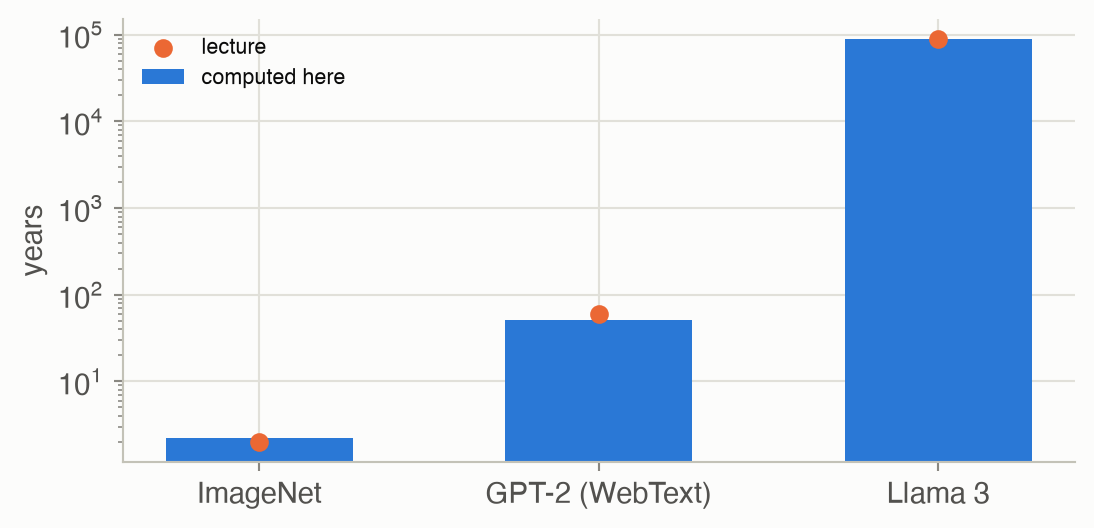
The lecture compares data sets by the time one person would need to get through them: about 2 years for ImageNet, 60 years for GPT-2’s training text, and 90,000 years for Llama 3’s ▶ 44:01. Those figures can be checked from published sizes plus a reading speed.
| data set | size (source) | assumption | years, non-stop | lecture |
|---|---|---|---|---|
| ImageNet | 14,197,122 images (image-net.org) | 5 s per image | 2.2 | 2 |
| GPT-2 (WebText) | 40 GB of text (Radford et al., 2019, Sec. 2.1) | 6 bytes per word, 250 words/min | 51 | 60 |
| Llama 3 | 15.6 trillion tokens (Llama Team, 2024) | 0.75 words per token, 250 words/min | 88,980 | 90,000 |
The reading speed and the bytes-per-word and words-per-token ratios are assumptions, so these are orders of magnitude, not exact figures; with them, all three come out within a factor of 2 of the lecture’s numbers. For scale on the robot side, the largest pooled robot data set the lecture shows, Open X-Embodiment, holds over a million trajectories, each one recorded episode of one robot (see Papers).
Interactive
Plan once, or look every step
Pick a position-estimate error. Each panel shows 20 episodes; the grey bars are the wall, with the doorway between them, and the circle is the goal. Crosses mark crashes.
What to try. At σ = 0 the closed-loop paths form one tight bundle through the doorway, while the sense-plan-act paths already spread out towards the goal: those are the motor errors adding up. Raise σ. The sense-plan-act paths shift as a whole, each copying the shape of the plan from a wrong starting point, and more of them end against the wall. The closed-loop paths wobble but keep converging on the doorway and the goal.
Precision of tokenized actions
Choose how many bins each action dimension gets. The chart shows, for every step of the 0.6 m reach, how far the robot is from the demonstrated path when it replays the tokens blindly (orange) or re-observes and tokenizes the correction (blue). The tokenization is recomputed in your browser.
What to notice. Each extra bit halves the bin width, and both curves shrink. The blue curve stays flat at the size of one rounding; the orange one wanders, because neighbouring moves round in the same direction and nothing corrects the sum. At 2 bits (4 bins) the blue curve is no longer the smaller one: with bins that coarse, the corrections themselves overshoot.
Algorithm & code
def tokenize(a, lo, hi, bins) -> Array:
    """Index of the bin each value falls in: [lo, hi] cut into `bins` equal
    bins; values outside are clipped to the end bins. Same shape as a."""
    k = np.floor((np.asarray(a) - lo) / (hi - lo) * bins).astype(int)
    return np.clip(k, 0, bins - 1)

def detokenize(k, lo, hi, bins) -> Array:
    """The centre of bin k: the value a token stands for."""
    return lo + (np.asarray(k) + 0.5) * (hi - lo) / bins

def replay(path, bins, closed_loop=False):
    """Execute the path's moves after a round trip through tokens.
    Open loop: tokenize the demonstrated moves and add them up.
    Closed loop: at each step tokenize the move from where the robot
    actually is to the next point on the path.
    Returns the executed path (T+1, 2)."""
    moves = np.diff(path, axis=0)                   # (T, 2) actions
    lo, hi = action_range(moves)                    # per-dimension range
    p, out = path[0].copy(), [path[0].copy()]
    for t in range(len(moves)):
        want = path[t + 1] - p if closed_loop else moves[t]
        p = p + detokenize(tokenize(want, lo, hi, bins), lo, hi, bins)
        out.append(p.copy())
    return np.array(out)
import numpy as np
import torch
import torch.nn as nn
import torch.nn.functional as F
from rlc.toys import w01_intro as toy
torch.manual_seed(0)
BINS, CTX = 256, 16
# Tokenize the reaching motion: (100, 2) moves -> (100, 2) integers.
moves = np.diff(toy.reach_path(), axis=0)
lo, hi = toy.action_range(moves)
tokens = torch.tensor(toy.tokenize(moves, lo, hi, BINS)) # int64
seq = tokens.reshape(-1) # (200,): x, y, x, y, ... like RT-2's ints
# Training windows: predict token j+1 from tokens up to j.
win = seq.unfold(0, CTX + 1, 1) # (185, CTX+1)
inputs, targets = win[:, :-1], win[:, 1:] # (185, CTX) each
class TinyActionGPT(nn.Module):
"""A decoder-only transformer over action tokens. A real VLA puts
image and instruction tokens in front of these in the same sequence."""
def __init__(self, vocab=BINS, d=64, ctx=CTX):
super().__init__()
self.tok = nn.Embedding(vocab, d)
self.pos = nn.Embedding(ctx, d)
layer = nn.TransformerEncoderLayer(d, nhead=4, dim_feedforward=128,
batch_first=True)
self.body = nn.TransformerEncoder(layer, num_layers=2)
self.head = nn.Linear(d, vocab)
def forward(self, idx): # idx: (N, L) int64
L = idx.shape[1]
h = self.tok(idx) + self.pos(torch.arange(L)) # (N, L, d)
# Causal mask: position j may only attend to positions <= j.
mask = nn.Transformer.generate_square_subsequent_mask(L)
return self.head(self.body(h, mask=mask, is_causal=True))
model = TinyActionGPT()
opt = torch.optim.Adam(model.parameters(), lr=3e-3)
losses = []
for _ in range(150):
logits = model(inputs) # (N, L, BINS)
# cross_entropy wants (N*L, BINS) logits and (N*L,) class indices
loss = F.cross_entropy(logits.reshape(-1, BINS), targets.reshape(-1))
opt.zero_grad()
loss.backward()
opt.step()
losses.append(loss.item())
assert logits.shape == (inputs.shape[0], CTX, BINS)
assert losses[-1] < losses[0] / 3The NumPy code is everything the page’s tokenizer does: a floor and a clip to get the token, a bin centre to get back. The PyTorch sketch goes one step further, training a small transformer to continue the reaching motion’s token sequence, which is the core of how RT-2 and its successors produce actions.
Papers
There are no discussion papers in Week 1. These are papers the lecture relies on.
Key papers from the lecture
Solved problems
1. Token precision. A robot’s end effector moves at most 2 cm per control step along each axis, and each axis is tokenized into 256 uniform bins over [−2 cm, 2 cm]. What is the largest rounding error per step, and how many tokens does one action with 3 position axes, 3 rotation axes and a gripper need?
TipSolution
Bin width \(\Delta = 4\,\text{cm} / 256 \approx 0.156\) mm; the largest error per axis is half of that, about 0.078 mm (Equation 4). One action needs one token per dimension: 3 + 3 + 1 = 7 tokens. RT-2 adds an eighth for “episode finished” (Sec. 3.2 of the paper).
2. Blind replay. Suppose every move of a 100-step motion rounds the same way, by \(+0.05\) mm along \(x\). How far off is the end of a blind replay? And with closed-loop correction?
TipSolution
Blind: the errors add up to \(100 \times 0.05 = 5\) mm. Closed loop: each step aims at the next point of the path from where the robot actually is, so the previous error is part of the correction; what remains after any step is one rounding, at most half a bin. Systematic rounding is the worst case for open loop and harmless for closed loop. In this page’s toy, rounding is partly systematic, which is why the open-loop error grows (Figure 8).
3. A plan made from a wrong start. A sense-plan-act robot believes it starts 0.3 to the left of where it really is. Ignoring motor noise, where does its executed path end, and does it get through a door 0.8 wide?
TipSolution
Executing the plan moves the robot by exactly the planned displacements, so the whole executed path is the planned path shifted 0.3 to the right: it ends 0.3 from the goal. At the door it passes 0.3 off the door’s centre line, inside the 0.4 half-width, so it gets through, but with only 0.1 to spare; add a little motor drift and it hits the frame. A closed-loop robot’s next estimate would show it is off course, and it would correct.
4. Is it a robot? Classify a dishwasher, a teleoperated surgical robot and a chatbot on a phone by the two tests from the lecture’s class discussion: does it change the physical world, and does it act on its own?
TipSolution
Dishwasher: changes the world (cleans dishes) and runs on its own, but only one fixed program in a fixed environment. Surgical robot: changes the world with great dexterity, but a surgeon makes every decision; it is teleoperated, like the 2007 PR1. Chatbot: reasons generally and acts autonomously in conversation, but has no body and changes nothing physical. Robot learning aims for all three at once: physical effect, autonomy, and generality.
5. Why the data are not i.i.d. A cleaning robot records (camera image, action) pairs while it works. Give two reasons these pairs are not independent and identically distributed samples.
TipSolution
Not independent: consecutive images are nearly identical, and each action determines the next image (Equation 2). Not identically distributed: change the policy and the robot visits different places, so the distribution of images changes; a policy trained on one robot’s data then meets different states when it acts itself. Week 3 shows how this makes small imitation errors snowball.
Recap
- Sense-plan-act needs an exact picture of the world. Why it matters: it explains both the success of factory robots and the falls of humanoids, and motivates closed-loop, learned policies.
- Feedback beats precision. In the doorway toy, re-estimating at every step kept success at 100% up to σ = 0.25, while planning once fell below half by σ ≈ 0.21. Why it matters: every policy in this course is a closed-loop controller.
- Moravec’s paradox: physical skill is the hard part, and its data is scarce. Why it matters: data collection is a theme of nearly every week, from demonstrations (Week 3) to human video (Week 3’s guest) to pooled data sets (Week 9).
- Write actions as tokens and robotics becomes sequence modeling. Why it matters: this is how vision-language-action models reuse web-scale pretraining (Weeks 7 and 9), at the cost of a small, controllable loss of precision.
- Robot data are not i.i.d. Why it matters: it is the root of compounding error in imitation (Week 3) and of the exploration problem in reinforcement learning (Weeks 4–5).
Cheat sheet & connections
| Name | Formula | Where |
|---|---|---|
| Supervised learning | \(\min_\theta \frac{1}{N}\sum_i \ell(f_\theta(x_i), y_i)\), i.i.d. data | Equation 1 |
| Robot loop | \(a_t \sim \pi(\cdot \mid o_t)\), \(s_{t+1} \sim p(\cdot \mid s_t, a_t)\) | Equation 2 |
| Open vs closed loop | \(\text{plan}_t(\hat{s}_0)\) vs \(\pi(\hat{s}_t)\) | Equation 3 |
| Tokenization | \(k = \lfloor (a - a_{\min})/\Delta \rfloor\), \(\lvert a - \hat{a} \rvert \le \Delta/2\) | Equation 4 |
| Sequence model | \(\prod_j p(k_j \mid \text{image}, \text{text}, k_{<j})\) | Equation 5 |
Common pitfalls.
- Treating robot data like a supervised data set. Consecutive samples are correlated, and the policy changes the distribution it is evaluated on.
- Assuming tokenized actions are exact. They are rounded to the bin centre; count the bins against the precision the task needs.
- Judging a robot demo without asking whether it was teleoperated.
Connections. Next week formalizes the robot loop as a Markov decision process. Week 3 is the first family of algorithms, imitation learning, and shows what the non-i.i.d. data cost; Weeks 4 and 5 are the second, reinforcement learning. The action tokens on this page return in Week 7, with RT-2’s bins and their compressed successor FAST, and the vision-language-action models built on them in Week 9. Week 12 reviews the whole course in one table. In the ADM Companion, Chapter 1 introduces decision making under uncertainty, the broader setting of the robot loop.
Resources
- Lecture: video (1:04:35)
- Slides: Official slides (ETH; password-protected) · Community rebuild (unofficial, student repo)
- Papers:
- Open X-Embodiment: Robotic Learning Datasets and RT-X Models (Open X-Embodiment Collaboration, 2024)
- RT-2: Vision-Language-Action Models Transfer Web Knowledge to Robotic Control (Brohan et al., 2023)
- Homework: hw1: PyTorch & NumPy tutorial