Week 3 · Imitation Learning
Lecture of 2 March 2026 · guest: Danfei Xu
Big picture
Where this week fits
Week 2 set up the language: a robot observes \(o_t\), picks an action \(a_t\) from a policy \(\pi(a_t \mid o_t)\), and the world moves to a new state. It did not say where a good policy comes from. This week gives the first and most direct answer: copy a person who already knows how. Weeks 4 and 5 give the other answer, learning from reward by trial and error. Several ideas from this week return later: expressive action distributions in Week 6 (generative models), histories and transformers in Week 7, and imitation at scale in the generalist robot policies of Week 9.
The question this week answers: how do you turn a set of expert demonstrations into a policy, and why does straightforward copying break down?
The key ideas at a glance
- Behavioral cloning (BC). Treat each demonstrated moment as a labelled example, “in this situation the expert did this”, and train a network to predict the expert’s action with ordinary supervised learning. It is simple and often works.
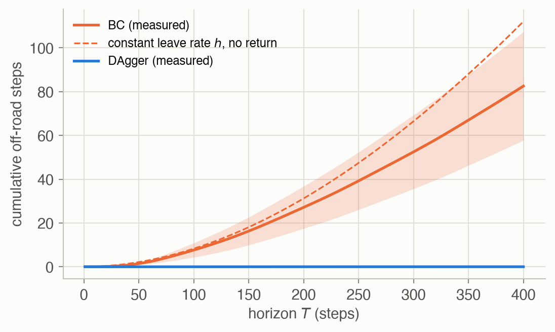
- Distribution shift and compounding error. Training data come from the states the expert visited; at test time the policy sees the states it visits. A small mistake leads to a state no demonstration covers, where the next mistake is more likely. If each step has a small chance \(\varepsilon\) of an unrecoverable mistake, the expected number of bad steps over a task of length \(T\) grows like \(\varepsilon T^2\), not \(\varepsilon T\).
- Show the policy how to recover. Either fake recovery data (side cameras labelled “steer back”), or run the policy, let an expert label the states it actually reaches, and retrain: DAgger. Letting a human take over only when the robot errs (human-gated DAgger) makes the labelling cheaper.
- Non-Markovian behavior and causal confusion. People act on memory and on things the robot cannot see. Feeding the policy a history helps in principle, but a high-capacity network may then latch onto a signal that merely correlates with the expert’s action instead of its cause.
- Multimodal behavior. When experts solve the same situation in different ways, a regression loss averages them, and the average of “left of the tree” and “right of the tree” is straight into it. Policies need distributions that can hold several peaks: mixtures of Gaussians, discretized actions, diffusion, or latent-variable models.
- From one task to any goal. Conditioning the policy on a goal, and learning from unscripted “play” data, turns imitation into a way to learn many skills at once.
Vocabulary
| Term | Plain meaning |
|---|---|
| Demonstration | A recorded run of an expert doing the task: the sequence of states (or observations) and actions |
| Expert policy \(\pi^*\) | The behavior being imitated, usually a person teleoperating the robot |
| Behavioral cloning (BC) | Supervised learning from (observation, expert action) pairs |
| Distribution shift | The states seen at test time differ from the states in the training data |
| Compounding error | Each mistake makes the next one more likely, so errors pile up over a trajectory |
| DAgger | Dataset Aggregation: label the learner’s own states with expert actions and retrain |
| Mode | One distinct way of doing the task, a peak of the action distribution |
| Causal confusion | The policy keys on a correlate of the expert’s action rather than its cause |
| Play data | Unscripted teleoperation with no fixed task, later relabelled with goals |
After this week you can
- Write down behavioral cloning as a loss and train it.
- Explain, with the \(\varepsilon T^2\) argument, why small imitation errors snowball, and how DAgger changes the bound to \(\varepsilon T\).
- Recognize when a policy needs a multimodal action distribution, and name four ways to build one.
- Spot non-Markovian demonstrations and the risk of causal confusion when adding history.
Intuition
TipAnalogy
Imagine learning to drive only by watching dashcam videos of a careful driver. Every frame shows the car in the middle of its lane, so you learn exactly what to do there. Then, on your first drive, a gust nudges you towards the verge. Nothing you watched shows a car near the verge, so you have no idea that you should steer back. The fix is not more videos of perfect driving. It is videos of recoveries, or an instructor who tells you what to do in the situations you get yourself into.
Copy what the expert did
Behavioral cloning is the dashcam student. You collect pairs: “the car was a little left of the centre line, heading slightly right, the road curving left: the expert steered a little left.” A network learns to map the first half of each pair to the second. The lecture introduces it as the most straightforward version of imitation learning ▶ 03:58. Formally it is a regression loss, Equation 1.
One slip and you are somewhere new
The road toy on this page makes the analogy concrete. The expert keeps the car’s heading along the road and, like most drivers, ignores small offsets from the centre line; only past 0.3 (in road half-widths of 1.0) does it steer back. Its demonstrations were recorded on a calm day, so the car never left that band and the data never show a steer-back. At deployment, each step has a 0.2% chance of a gust that turns the car by 0.4 rad.
What to watch for. All the cars start together on the centre line and stay together until the gust: before it, the cloned policies drive as well as the expert. The gust pushes every car towards the edge by about the same amount. From there the colours separate. The black expert and the blue DAgger cars turn back into the road. The orange clones fan out: some steer back by luck, some drift across the edge, and some turn sharply away, because nothing in their calm-day data said what to do there.
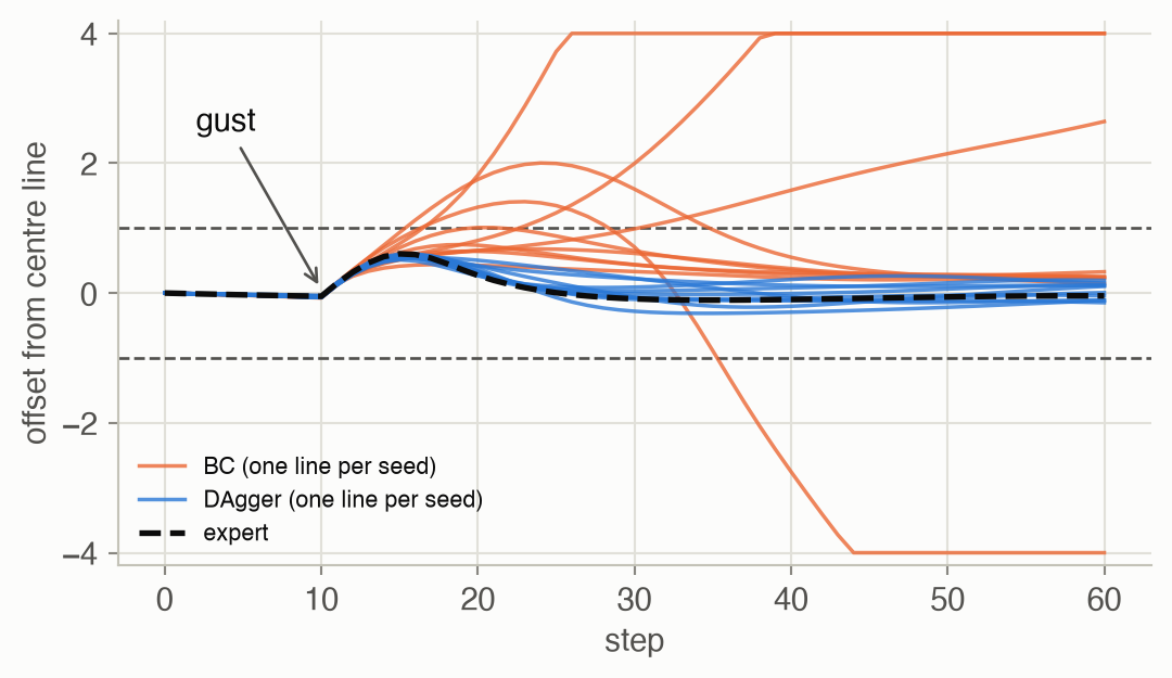
The gust pushes every car out by about the same amount at first. The expert’s offset peaks at 0.60, past its deadband, and it steers back. The cloned policies split. They were trained only on near-centre states, so what each does further out is an accident of its training run: of the 10 BC policies, 6 happen to steer back, 4 end off the road, and 3 of those end more than five units from the centre line. This is the lecture’s tightrope walker: once you fall off, no demonstration shows how to get back on ▶ 15:16. The general version is distribution shift: the states the policy visits stop matching the states the expert visited ▶ 06:18. The formal cost of it is Equation 2.
Ask the expert about your own mistakes
If the problem is missing recovery data, supply it. NVIDIA’s self-driving car added two side cameras and labelled their images “steer right” and “steer left”, which creates recovery examples without ever crashing ▶ 12:01. DAgger does the same thing systematically: drive with the current policy, ask the expert what it would have done at each state the policy reached, add those pairs to the data, and retrain ▶ 18:44. In the road toy, DAgger’s policies (blue above) have seen post-gust states labelled with the expert’s steer-back, and every one of them recovers. Asking an expert to relabel thousands of states afterwards is tedious, so in practice a human often watches and takes over only when the robot is about to fail (human-gated DAgger) ▶ 20:48. The formal version is Equation 3.
What the expert knew that the robot didn’t
Experts are not Markovian: a driver brakes because of how a cyclist moved over the last few seconds, and a teleoperator sees the scene from angles the robot’s camera does not ▶ 25:38. Giving the policy a history of observations is the obvious fix. It can backfire. In the lecture’s drawer example, the demos always show a 10 N force spike when the gripper grasps the handle, so the network learns “pull when the force reads 10 N” instead of “pull when the handle is grasped”; if the gripper slips and reads 2 N, it never pulls ▶ 29:56. This is causal confusion, the subject of one of this week’s papers.
Two good answers can average to a bad one
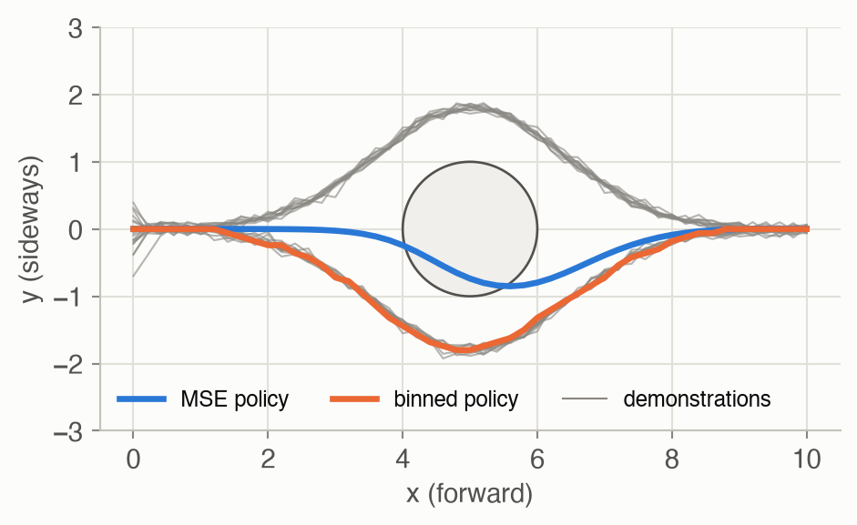
Real demonstrations rarely agree on one way to do a task: there are endless ways to close a drawer, and different operators pick different ones ▶ 32:11. A mean-squared-error loss is minimized by the average action, and the average of two good routes around a tree is straight into the tree ▶ 33:46. In this toy, with half the demos passing on each side, the MSE policy hit the obstacle in 50% of 20 training seeds and the binned policy in 0%. The fix is a policy that outputs a distribution able to hold several peaks ▶ 34:41: see Equation 4, Equation 5, and the latent-variable model in Equation 6.
From one task to any goal
Task labels are a blunt instrument: is a sliding door moved halfway “opened”? The lecture argues for goal-conditioned policies, \(\pi(a_t \mid s_t, s_g)\), that learn to reach any goal state from any start, and for play data: operators teleoperate the robot freely, with no task, and every window of that data is relabelled with its own final frame as the goal ▶ 43:37. Play data are cheap and diverse, but highly multimodal, which is why the lecture pairs them with a latent-variable policy (Equation 6).
Key concepts & formulae
The lecture’s notation: \(s_t\) is the state, \(o_t\) the observation, \(a_t\) the action at time \(t\); \(\pi^*\) is the expert and \(\pi_\theta\) the learned policy with parameters \(\theta\); \(\mathcal{D}\) is the demonstration data set. ADM Chapter 18 writes the expert as \(\pi_E\).
Behavioral cloning
\[ \theta^\star = \arg\min_\theta \; \frac{1}{|\mathcal{D}|} \sum_{(s, a^*) \in \mathcal{D}} \big\lVert \pi_\theta(s) - a^* \big\rVert^2 \tag{1}\]
In words. Pick the network weights that make the policy’s action as close as possible, on average, to what the expert did in the same state.
Term by term.
- \(\mathcal{D}\): every (state, expert action) pair from every demonstration, pooled; the trajectory structure is thrown away.
- \(\pi_\theta(s)\): the policy’s action in state \(s\), a deterministic network output here.
- \(a^*\): the action the expert took in that state.
- \(\lVert\cdot\rVert^2\): squared error, summed over action dimensions. Any regression or classification loss can stand here; the next sections replace it.
Why it holds: MSE predicts the average. For a fixed state, the number \(c\) that minimizes \(\mathbb{E}[(c - a^*)^2]\) over the expert’s possible actions satisfies \(\frac{d}{dc}\mathbb{E}[(c-a^*)^2] = 2(c - \mathbb{E}[a^*]) = 0\), so \(c = \mathbb{E}[a^* \mid s]\): the mean of the actions the expert took there. That is fine when the expert is consistent and disastrous when it is not.
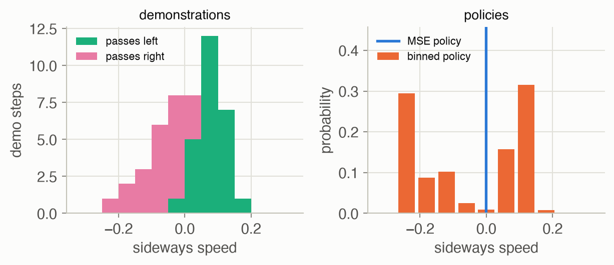
Quick check. In the obstacle toy, the demonstrated sideways speeds near the fork \((x, y) = (2, 0)\) have mean +0.011 (from 48 demo steps, 28 steering left and 20 right). The MSE network outputs -0.001 there: close to that average, and close to neither group’s action.
Distribution shift and the \(\varepsilon T^2\) bound
BC minimizes its loss on states drawn from \(p_{\text{expert}}(s)\), the states the expert visits. What matters at test time is how it does on \(p_{\pi_\theta}(s)\), the states it visits. These differ as soon as the policy makes a mistake.
\[ \begin{aligned} c(s, a) &= \begin{cases} 0 & a = \pi^*(s) \\ 1 & \text{otherwise} \end{cases} \\ \Pr\big(\pi_\theta(s) \neq \pi^*(s)\big) &\le \varepsilon \quad (s \sim p_{\text{expert}}) \\[4pt] \mathbb{E}\Big[\sum_{t=1}^{T} c(s_t, a_t)\Big] &\le \varepsilon T \\ &\quad + (1-\varepsilon)\big(\varepsilon (T-1) + \dots\big) \\ &= O(\varepsilon T^2) \end{aligned} \tag{2}\]
In words. If the cloned policy errs with probability at most \(\varepsilon\) on the expert’s states, but an error takes it to states where it can no longer be trusted, its expected number of mistakes over \(T\) steps can grow with \(T^2\).
Term by term.
- \(c(s, a)\): the cost of a step, 1 if the policy’s action differs from the expert’s.
- \(\varepsilon\): the mistake rate on states the expert visits, which is what supervised training controls.
- \(T\): the task length in steps.
- \(\varepsilon T\): the cost of a first mistake at step 1, paid on all \(T\) steps (the tightrope: once off, always off).
- \((1-\varepsilon)\,\varepsilon(T-1)\): no mistake at step 1, first mistake at step 2, paid on the remaining \(T-1\) steps; and so on.
Why it holds. A first mistake at step \(t\) costs at most \(T - t + 1\), and happens with probability at most \(\varepsilon\). Summing, \(\sum_{t=1}^{T} \varepsilon (T - t + 1) = \varepsilon \frac{T(T+1)}{2}\), which is \(O(\varepsilon T^2)\). Compare supervised learning on independent examples, where \(T\) predictions cost \(\varepsilon T\). The analysis is from Ross et al. (2011), cited in the lecture ▶ 15:16.
Numeric check. In the road toy, over 16 seeds × 200 cars, BC’s mean cumulative off-road steps are 1.5, 7.6, 27.1 and 82.5 at \(T =\) 50, 100, 200 and 400: a slope of 1.93 on a log-log scale, close to the quadratic’s 2. The measured rate at which an on-road BC car leaves is 0.0017 per step. If departures were permanent, that rate would predict 112 off-road steps by \(T = 400\); the toy measures 83, lower because 35% of the cars that left were back on the road at the end. DAgger’s policies, facing the same gusts, total 0.013.
DAgger: label the learner’s own states
\[ \begin{aligned} \mathcal{D} &\leftarrow \mathcal{D} \cup \big\{ (s, \pi^*(s)) : s \sim p_{\pi_\theta} \big\} \\ \theta &\leftarrow \arg\min_\theta \mathcal{L}(\pi_\theta, \mathcal{D}) \end{aligned} \tag{3}\]
In words. Collect states by running the current learned policy, label each with the expert’s action, add them to everything collected so far, and refit.
Term by term.
- \(s \sim p_{\pi_\theta}\): states drawn from the learner’s own trajectories, mistakes included. This is the distribution BC never trains on.
- \(\pi^*(s)\): the expert’s label, “what I would do here”. The expert does not have to drive; it only has to answer.
- \(\mathcal{D} \cup\): the old data are kept, so the policy does not forget earlier states (aggregation, the “Agg” in DAgger).
- \(\mathcal{L}\): the same supervised loss as BC, for example Equation 1.
Why it helps. After enough rounds the training data cover the states the policy itself reaches, so the mistake rate \(\varepsilon\) holds where the policy actually is. A mistake no longer leads into unknown territory, and the bound drops from \(O(\varepsilon T^2)\) to \(O(\varepsilon T)\) (Ross et al., 2011). The cost is an expert who can be queried on states it did not choose, which the lecture flags as slow and costly in practice ▶ 19:55.
Expressive action distributions
When the expert’s action in a state has several modes, the policy must output a distribution \(\pi_\theta(a \mid s)\) rather than a single action, and be trained by maximum likelihood instead of squared error.
\[ \pi_\theta(a \mid s) = \sum_{k=1}^{K} w_k(s)\, \mathcal{N}\big(a;\, \mu_k(s), \Sigma_k(s)\big) \tag{4}\]
In words. The network outputs \(K\) bell curves and a weight for each; the action is drawn from their weighted sum.
Term by term.
- \(K\): the number of components, fixed in advance; the lecture notes this as the main limitation ▶ 34:41.
- \(w_k(s)\): how likely mode \(k\) is in state \(s\); a softmax output, so the weights sum to 1.
- \(\mu_k(s), \Sigma_k(s)\): the centre and spread of mode \(k\).
In the obstacle toy, two components would do: one centred on “steer left”, one on “steer right”, each with weight near one half at the fork.
\[ p(a_t \mid s_t) = \prod_{d=1}^{D} p\big(a_{t,d} \mid s_t, a_{t,1}, \dots, a_{t,d-1}\big) \tag{5}\]
In words. Split the action into its \(D\) dimensions, chop each into bins, and predict the bins one dimension at a time, each conditioned on the ones already chosen.
Term by term.
- \(a_{t,d}\): the bin chosen for dimension \(d\) (a class label), trained with cross-entropy.
- The product: the chain rule of probability, exact for any joint distribution.
- Why not one big grid: with \(D\) dimensions of \(B\) bins each, a joint grid has \(B^D\) classes; the product needs only \(D\) predictions of \(B\) classes each ▶ 35:27. This is how the first vision-language-action models emitted actions, as tokens from a transformer (Weeks 7 and 9).
The binned policy in the obstacle toy is the one-dimensional case, \(D = 1\) with 11 bins. At the fork its probabilities put 0.48 on the left-steering bins and 0.51 on the right-steering bins (Figure 6).
The lecture also previews diffusion policies, which turn noise into an action by repeated denoising and are the subject of Week 6 ▶ 37:32, and latent-variable policies, which receive an extra random input \(z\) that selects the mode ▶ 39:22. For the latter, the training objective is the evidence lower bound.
\[ \begin{aligned} \log p_\theta(\tau \mid c) \;\ge\;\; & \mathbb{E}_{q_\phi(z \mid \tau, c)}\big[\log p_\theta(\tau \mid z, c)\big] \\ -\; & \mathrm{KL}\big(q_\phi(z \mid \tau, c)\,\big\|\,p(z \mid c)\big) \end{aligned} \tag{6}\]
In words. We would like to maximize the likelihood of the demonstrated trajectory, but that requires averaging over every possible latent plan \(z\). Instead, maximize a lower bound: reconstruct the trajectory well from a plan inferred from it, while keeping that inferred plan close to what could be proposed from the start and goal alone.
Term by term.
- \(\tau\): a short window of demonstration (states and actions); \(c = (s_c, s_g)\): its context, the current state \(s_c\) and the goal \(s_g\).
- \(z\): a latent plan, a continuous vector that picks one way of getting from \(s_c\) to \(s_g\).
- \(q_\phi(z \mid \tau, c)\): the posterior (“plan recognition”), which sees the whole window and infers which plan it followed.
- \(p_\theta(\tau \mid z, c)\): the action decoder, the policy itself, rewarded for reproducing the window’s actions given the plan.
- \(p(z \mid c)\): the prior (“plan proposal”), which sees only start and goal. The KL term pulls the recognized plans and the proposed plans together, so at test time the prior alone can propose plans.
Why it holds. For any distribution \(q\) over \(z\), \(\log p(\tau \mid c) = \log \mathbb{E}_{q}\big[p(\tau, z \mid c)/q(z)\big]\), which by Jensen’s inequality (\(\log\) is concave) is at least \(\mathbb{E}_q\big[\log p(\tau, z \mid c) - \log q(z)\big]\); splitting \(p(\tau, z \mid c) = p(\tau \mid z, c)\, p(z \mid c)\) gives the two terms. Because the plan absorbs the choice between modes, the decoder only has to model one mode at a time, as the lecture puts it ▶ 46:22.
Worked examples
Example 1: a gust, step by step
The table follows three cars of Figure 2 from just before the gust: the expert, the BC policy that ends farthest off the road (seed 5), and the DAgger policy of the same seed. Offsets are signed distances from the centre line; the road edge is at 1.0.
| step | expert | BC | DAgger |
|---|---|---|---|
| 10 | -0.05 | -0.08 | -0.04 |
| 11 | +0.15 | +0.12 | +0.16 |
| 12 | +0.32 | +0.30 | +0.32 |
| 14 | +0.56 | +0.62 | +0.51 |
| 17 | +0.54 | +1.09 (off) | +0.50 |
| 20 | +0.27 | +1.82 (off) | +0.32 |
| 30 | -0.09 | +5.98 (off) | -0.10 |
| 45 | -0.08 | +13.21 (off) | -0.11 |
| 60 | -0.04 | +20.43 (off) | +0.01 |
For the first steps after the gust the three cars move alike: each straightens its heading, which the calm-day data did teach. They part once the offset passes the expert’s deadband at 0.3, a region no demonstration covered. The expert starts steering back, the DAgger policy (trained on such states) does the same, and this BC policy, left to guess, keeps going.
How much DAgger data does it take? Averaged over the 16 seeds, the share of cars that leave the road at least once in 400 steps:
| policy | cars that leave the road |
|---|---|
| BC | 54.2% |
| DAgger, round 1 | 3.7% |
| DAgger, round 2 | 0.5% |
| DAgger, round 3 | 0.5% |
| DAgger, round 4 | 0.4% |
One round of relabelled data does most of the work: the policy sees what happens after a gust once, and the expert’s labels fill the gap. Later rounds add little, because the policy now rarely reaches new states.
The averages hide a wide spread between seeds. With the same calm-day demos, BC’s cumulative off-road steps at \(T = 400\) ranged from 0 to 354 across seeds, and in 6 of the 16 seeds BC left the road even with no gusts at all. A network trained only on near-centre states has to guess what to do elsewhere, and each seed guesses differently: some guesses happen to steer back, some drift. That unpredictability is the practical face of distribution shift.
Example 2: the fork
At the fork \((x, y) = (2, 0)\), half the demos are about to swing left and half right. The left panel shows the sideways speeds the demos actually used near that point; the right panel shows what each learned policy does there.
| bin centre (sideways speed) | binned policy’s probability |
|---|---|
| -0.30 | 0.00 |
| -0.24 | 0.29 |
| -0.18 | 0.09 |
| -0.12 | 0.10 |
| -0.06 | 0.03 |
| +0.00 | 0.01 |
| +0.06 | 0.16 |
| +0.12 | 0.32 |
| +0.18 | 0.01 |
| +0.24 | 0.00 |
| +0.30 | 0.00 |
The MSE policy outputs -0.001: go straight, the average of two groups that lean opposite ways. The binned policy puts 0.48 of its probability on steering left and 0.51 on steering right, and taking the most likely bin commits it to one side. One step later the robot is no longer at \(y = 0\), the demos near its new position all agree, and the choice sticks.
Interactive
Drift under gusts
Move the slider to change how often gusts hit. Each panel shows 20 cars driven by one policy, as offset from the centre line over 400 steps; the dashed lines are the road edges. The policies are from one seed, chosen by an explicit rule: among seeds whose BC car never leaves the road on a calm day, the one whose BC cost is closest to their median (seed 6).
What to try. Start at 0%: with no gusts every car of both policies stays inside the edges. Raise the rate. In the top panel, more and more BC cars cross an edge: at 1% per step, 75% of the 20 cars leave the road at some point, and a BC car spends on average 21.7 of its 400 steps off it. In the bottom panel, DAgger’s cars spike towards the edge after each gust and come back: 15% cross an edge at all, for 0.3 steps per car on average. This seed’s BC policy is a middling one: 0% of its cars are still off the road at step 400, so its departures are long detours rather than the permanent ones of the worst seeds in Figure 2.
Demonstration modes
Slide the share of demonstrations that pass on the left, and pick one of three training seeds. Grey: the 20 demonstrations; blue: the MSE policy; orange: the binned policy. Both policies are retrained for every setting.
What to notice. At 0 or 1, all demos agree and both policies follow them. Near an even split, the blue path is pulled between the two bundles: across the three seeds the MSE policy hits the obstacle at shares 0.4 and 0.5 (5 of the 33 settings in all). The binned policy hits it in 0 of them. It always commits to one side; in 1 of the settings with an uneven split it picks the side fewer demos chose, which is still a valid way around.
Algorithm & code
Behavioral cloning and DAgger
def fit_policy(obs, actions, rng, epochs=300, hidden=32):
    """MLP from scaled observations to steering. Returns a batch policy
    (n, 3) -> (n,)."""
    X = obs / SCALE                         # (m, 3), each feature O(1)
    net = nn.init_mlp([3, hidden, hidden, 1], rng)
    params, _ = nn.fit(net, X, actions[:, None], "mse", "tanh",
                       alpha=0.01, epochs=epochs, rng=rng)
    return lambda o: nn.predict(params, o / SCALE)[:, 0]

def behavior_cloning(n_demos, T, rng):
    obs, act = expert_data(n_demos, T, rng)
    return fit_policy(obs, act, rng)

def dagger(n_demos, T, rng, eps=EPS, iters=4, stride=4, history=False):
    """Start from BC on the calm-day demos; then repeatedly drive the current
    policy at deployment (gusts included), ask the expert what it would have
    done at each visited state, add those (state, expert action) pairs, and
    refit on everything. Only every `stride`-th visited state is kept:
    neighbouring states are nearly identical, and fewer points fit faster.
    history=True returns the policy after every round, BC first."""
    obs, act = expert_data(n_demos, T, rng)
    policies = [fit_policy(obs, act, rng)]
    for _ in range(iters):
        starts = rng.uniform(0, WAVELEN, n_demos)
        _, new = rollout(policies[-1], T, eps, rng, starts)
        new = new[:, ::stride].reshape(-1, 3)    # (n_demos * T/stride, 3)
        obs = np.vstack([obs, new])
        act = np.concatenate([act, expert(new)])  # the expert relabels
        policies.append(fit_policy(obs, act, rng))
    return policies if history else policies[-1]
import numpy as np
import torch
import torch.nn as nn
import torch.nn.functional as F
from rlc.toys import w03_imitation as road # the road toy on this page
torch.manual_seed(0)
rng = np.random.default_rng(0)
SCALE = torch.tensor(road.SCALE, dtype=torch.float32)
# Calm-day demos: obs (N, 3) = (offset, heading error, road turn),
# act (N,) = the expert's steering.
obs, act = road.expert_data(n_demos=10, T=200, rng=rng)
X = torch.tensor(obs, dtype=torch.float32) / SCALE # (N, 3)
y = torch.tensor(act, dtype=torch.float32)[:, None] # (N, 1)
policy = nn.Sequential(nn.Linear(3, 32), nn.Tanh(),
nn.Linear(32, 32), nn.Tanh(), nn.Linear(32, 1))
opt = torch.optim.Adam(policy.parameters(), lr=1e-2)
def train(X, y, steps):
"""Full-batch BC: regress the expert's action. Returns the losses."""
losses = []
for _ in range(steps):
loss = F.mse_loss(policy(X), y) # behavior cloning = regression
opt.zero_grad() # .grad accumulates otherwise
loss.backward()
opt.step()
losses.append(loss.item())
return losses
losses = train(X, y, steps=300)
assert losses[-1] < losses[0] / 10def as_numpy_policy(net):
"""Wrap the network for road.rollout: (n, 3) array -> (n,) array."""
def act_fn(o):
with torch.no_grad(): # acting needs no gradients
x = torch.tensor(o, dtype=torch.float32) / SCALE
return net(x)[:, 0].numpy()
return act_fn
# DAgger: drive the current policy, let the expert label what it saw.
for _ in range(2):
starts = rng.uniform(0, road.WAVELEN, 10)
# Gust rate 1% (page: 0.2%) so two short rounds meet enough gusts.
_, seen = road.rollout(as_numpy_policy(policy), 200, 0.01, rng, starts)
seen = seen[:, ::4].reshape(-1, 3) # (10 * 50, 3)
labels = road.expert(seen) # "here I would do this"
X = torch.cat([X, torch.tensor(seen, dtype=torch.float32) / SCALE])
y = torch.cat([y, torch.tensor(labels, dtype=torch.float32)[:, None]])
train(X, y, steps=200) # refit on all data
assert X.shape == (2000 + 2 * 500, 3) and y.shape == (3000, 1)The only difference between the two algorithms is the loop: BC trains once on the expert’s states; DAgger keeps adding the learner’s states, labelled by the expert (expert(new) in the NumPy version), and refits on everything.
A policy that can hold two modes
def fit_mse(obs, acts, rng, epochs=400):
    """Regression: one sideways velocity per observation, MSE loss. Where
    demos disagree, MSE is minimized by their average."""
    net = nn.init_mlp([2, 32, 32, 1], rng)
    params, _ = nn.fit(net, obs / SCALE2, acts[:, None], "mse", "tanh",
                       alpha=0.01, epochs=epochs, rng=rng)
    return lambda o: nn.predict(params, o / SCALE2)[:, 0]

def to_bin(acts) -> Array:
    """Index of the nearest bin centre, (n,) ints."""
    return np.abs(acts[:, None] - BINS[None, :]).argmin(axis=1)

def fit_binned(obs, acts, rng, epochs=400):
    """Classification over BINS with cross-entropy. The network outputs a
    probability for every bin, so two modes stay two peaks. The policy takes
    the most likely bin."""
    net = nn.init_mlp([2, 32, 32, len(BINS)], rng)
    params, _ = nn.fit(net, obs / SCALE2, to_bin(acts), "cross_entropy",
                       "tanh", alpha=0.01, epochs=epochs, rng=rng)
    # (n, 2) -> (n, len(BINS)): one probability per bin, rows sum to 1
    probs = lambda o: nn.softmax(nn.predict(params, o / SCALE2))
    policy = lambda o: BINS[probs(o).argmax(axis=1)]
    return policy, probs
from rlc.toys.w03_imitation import (BINS, SCALE2, demos2, hits, rollout2,
to_bin)
_, obs2, acts2 = demos2(20, 0.5, rng) # half left, half right
X2 = torch.tensor(obs2 / SCALE2, dtype=torch.float32) # (1000, 2)
target = torch.tensor(to_bin(acts2)) # (1000,) int64 bins
binned = nn.Sequential(nn.Linear(2, 32), nn.Tanh(),
nn.Linear(32, 32), nn.Tanh(),
nn.Linear(32, len(BINS))) # one logit per bin
opt2 = torch.optim.Adam(binned.parameters(), lr=1e-2)
losses2 = []
for _ in range(400):
# cross_entropy takes raw logits (N, K) and class indices (N,);
# it applies log-softmax itself, so no softmax layer in the network.
loss = F.cross_entropy(binned(X2), target)
opt2.zero_grad()
loss.backward()
opt2.step()
losses2.append(loss.item())
def most_likely_bin(o):
"""(n, 2) positions -> (n,) sideways speeds: the centre of the top bin."""
with torch.no_grad():
logits = binned(torch.tensor(o / SCALE2, dtype=torch.float32))
return BINS[logits.argmax(dim=-1).numpy()] # argmax over bins
path, _ = rollout2(most_likely_bin) # (1, 51, 2)
assert losses2[-1] < losses2[0] / 2
assert not hits(path)[0] # it commits to one side and clears it
assert abs(path[0, 25, 1]) > 1.0 # at x = 5 it is well off to one sideThe binned network differs from the MSE one in two places: its last layer has one output per bin instead of one number, and its loss is cross-entropy over bin indices instead of squared error. Everything else, including the data, is identical.
Papers
Papers discussed in class
Key papers from the lecture
Guest spotlight
Danfei Xu (Georgia Tech) argues that robot learning should get its data the way language and vision models do: from people going about their lives, not only from people teleoperating robots ▶ 01:32. He frames robot learning as a triangle of data source, learning algorithm and physical system, and argues that changing one corner means redesigning the other two ▶ 02:07. Teleoperation ties all three together: data exist only where a person drives a particular robot, and the resulting policy works only on that robot.
His group’s EgoMimic records people doing tasks while wearing Meta’s Project Aria glasses, then treats human hands as one more embodiment alongside the robot’s arms and co-trains a single behavioral cloning policy on both ▶ 06:18. The robot even wears the same glasses as its camera, to shrink the viewpoint gap. In his scaling experiment, more teleoperation data improved the robot only gradually, while adding human data on top of a fixed amount of robot data gave a sharp jump; he also reports that people demonstrate some tasks up to ten times faster than teleoperators ▶ 11:27.
Co-training alone does not make human and robot data share a representation; inside the network they stayed in two separate clusters. EgoBridge adds a loss, based on optimal transport, that pulls the two distributions together while keeping their action structure, so that a task shown only in human data can transfer to the robot ▶ 15:11. The talk closes with EMMA, which extends the approach to mobile manipulation, and EgoVerse, a shared human-data set of about 1,300 hours at the time of the talk ▶ 29:11.
How it connects to this week. Every method in the talk builds on behavioral cloning; what changes is where \(\mathcal{D}\) comes from. Human data from wearable cameras is cheap and plentiful, but it is a different distribution from what the robot sees and does, which is this week’s distribution-shift problem at the level of the whole data set rather than a single trajectory.
Solved problems
1. The bound, with numbers. A cloned policy makes an unrecoverable mistake with probability \(\varepsilon = 0.01\) per step on the expert’s states. For a task of \(T = 100\) steps, compare the BC bound with the \(\varepsilon T\) you would expect from independent predictions.
TipSolution
Independent predictions: \(\varepsilon T = 0.01 \times 100 = 1\) expected mistake. The BC bound from Equation 2: \(\varepsilon \frac{T(T+1)}{2} = 0.01 \times \frac{100 \times 101}{2} = 50.5\) expected bad steps, fifty times more. If departures are permanent and the rate is exactly \(\varepsilon\), the expected cost is \(\sum_{t=1}^{100} \big(1 - 0.99^t\big) = 100 - 0.99 \cdot \frac{1 - 0.99^{100}}{0.01} \approx\) 37.2; the bound is looser because a car that has already left cannot leave again. Both are far above 1, and the gap grows with \(T\).
2. A lopsided fork. At the fork in the obstacle toy, suppose 70% of demonstrators steer left at \(+0.3\) and 30% steer right at \(-0.3\). What does a perfectly trained MSE policy output, and what does a binned policy that takes the most likely bin output?
TipSolution
MSE outputs the mean (Equation 1): \(0.7 \times 0.3 + 0.3 \times (-0.3) = 0.12\), a gentle left turn that no demonstrator made. Whether that clears the obstacle depends on whether the robot gets far enough to the side in time; set the explorer’s share to 0.7 and compare the seeds. The binned policy puts probability 0.7 on the \(+0.3\) bin and 0.3 on the \(-0.3\) bin and takes \(+0.3\): a real demonstrated action. Sampling from the bins instead would go right 30% of the time, also a valid way around.
3. Recovery labels without an expert in the loop. The NVIDIA car labels its left camera’s images “steer right”. Why does that produce the same kind of data DAgger collects, and what can it not provide?
TipSolution
The left camera sees the road as it would look if the car had drifted left: an off-centre state the expert never drove through. Labelling it “steer right” gives a (state, corrective action) pair, exactly what DAgger obtains by driving the learner and asking the expert. It is limited to the drifts the camera geometry simulates (a fixed sideways shift) and to a correction rule chosen by the engineer rather than an expert’s judgement; larger or different mistakes, such as the heading errors after a gust in the road toy, remain uncovered. DAgger covers whatever states the policy actually reaches.
4. Grids versus chains. A 7-dimensional arm action is discretized into 256 bins per dimension. How many classes does a joint grid need, and how many outputs does the autoregressive factorization (Equation 5) need?
TipSolution
Joint grid: \(256^7 = 2^{56} \approx 7.2 \times 10^{16}\) classes, impossible to train a softmax over. Autoregressive: 7 predictions of 256 classes each, 1,792 logits in total, produced one dimension at a time. The price is sequential decoding: 7 forward passes (or 7 steps of a transformer) per action.
5. Spot the causal confusion. A driving policy sees the camera image and the previous action. In the demos, the car brakes at red lights and keeps braking for several frames. The cloned policy brakes well when started at a red light but never starts braking on its own. What went wrong?
TipSolution
In the data, “previous action was brake” predicts “brake now” almost perfectly, far better than the small red light in the image does. The network learns to copy its previous action, a correlate, not the cause (the light). At test time nothing ever starts the braking chain. Remedies follow the papers: remove or randomly drop the previous-action input, or test which input the policy should rely on with a few targeted interventions (de Haan et al., 2019).
Recap
- Behavioral cloning is supervised learning on expert (state, action) pairs. Why it matters: it is the baseline every imitation method improves on, and at large scale it is the training recipe of the generalist policies in Week 9.
- A cloned policy is tested on its own states, not the expert’s. Small mistakes lead to unseen states, and the expected cost can grow like \(\varepsilon T^2\); on the road toy it grew with slope 1.9 on a log-log scale. Why it matters: this is why “lower training loss” does not guarantee a better robot.
- Recovery data fix it. Synthetic corrections (side cameras), DAgger’s relabelled states, or human interventions all show the policy how to get back. Why it matters: it reframes data collection: mistakes and recoveries are valuable data.
- Experts are not consistent, and MSE averages their choices. Policies need multimodal action distributions: mixtures, discretization, diffusion, latent plans. Why it matters: Week 6’s diffusion policies and Week 7’s token-based policies are answers to exactly this.
- More inputs can hurt. History and extra sensors invite causal confusion. Why it matters: it explains why later policies are careful about what context they condition on.
Cheat sheet & connections
| Name | Formula | Where |
|---|---|---|
| BC loss | \(\min_\theta \sum_{\mathcal{D}} \lVert \pi_\theta(s) - a^* \rVert^2\) | Equation 1 |
| MSE minimizer | \(c^\star = \mathbb{E}[a^* \mid s]\) | Equation 1 |
| BC compounding error ★ | \(\mathbb{E}[\sum_t c] = O(\varepsilon T^2)\) | Equation 2 |
| DAgger data rule, cost \(O(\varepsilon T)\) | \(\mathcal{D} \leftarrow \mathcal{D} \cup \{(s, \pi^*(s))\}\), \(s \sim p_{\pi_\theta}\) | Equation 3 |
| Mixture of Gaussians | \(\sum_k w_k \mathcal{N}(a; \mu_k, \Sigma_k)\) | Equation 4 |
| Autoregressive actions | \(\prod_d p(a_{t,d} \mid s_t, a_{t,<d})\) | Equation 5 |
| ELBO ★ | \(\mathbb{E}_q[\log p(\tau \mid z, c)] - \mathrm{KL}(q \Vert p)\) | Equation 6 |
Common pitfalls.
- Judging a cloned policy by its validation loss on held-out demos. Those are still expert states; only closed-loop rollouts measure distribution shift.
- Collecting only clean, perfect demonstrations. They teach nothing about recovery.
- Using MSE when demonstrators disagree. Check for multiple modes before choosing the loss.
- Adding history “because it can only help”. It can hurt through causal confusion.
Connections. Week 2 gave the policy and MDP vocabulary used here. Weeks 4–5 learn from reward instead of demonstrations. Week 6 builds diffusion policies, the most common answer to multimodality today. Week 7 turns actions into token sequences, the autoregressive factorization above. Week 9’s generalist policies are trained largely by behavioral cloning, at scale. In the ADM Companion: behavioral cloning and DAgger in tabular settings, plus inverse reinforcement learning, which this lecture does not cover.
Resources
- Lecture: video (50:37)
- Slides: Official slides (ETH; password-protected) · Community rebuild (unofficial, student repo)
- Guest lecture: Danfei Xu (Georgia Tech), Human Data as a Foundation for Robot Learning: video (36:48)
- Papers:
- Causal Confusion in Imitation Learning (de Haan, Jayaraman & Levine, 2019)
- The Surprising Effectiveness of Representation Learning for Visual Imitation (Pari, Shafiullah, Arunachalam & Pinto, 2022)
- Transporter Networks: Rearranging the Visual World for Robotic Manipulation (Zeng et al., 2020)
- A Reduction of Imitation Learning and Structured Prediction to No-Regret Online Learning (Ross, Gordon & Bagnell, 2011)
- End to End Learning for Self-Driving Cars (Bojarski et al., 2016)
- Learning Latent Plans from Play (Lynch et al., 2019)
- Homework: hw3: Imitation learning