Week 5 · Reinforcement Learning II
Lecture of 16 March 2026 · guest: Andrew Wagenmaker
Big picture
Where this week fits
Week 4 learned what every action is worth, a Q-function, and acted by taking the best one. That needs a maximum over actions, which is hard when actions are continuous and high-dimensional ▶ 01:30. This week skips the detour: give the policy parameters \(\theta\) and adjust them directly, so that actions which led to high reward become more likely ▶ 02:02. These are policy-gradient methods. The lecture builds them up one fix at a time, from the simplest (REINFORCE) to the two algorithms most used in robotics today, PPO and SAC, and ends by bringing value functions back as critics.
The question this week answers: how do you follow the gradient of expected reward when you cannot differentiate through the world, and how do you make that gradient precise and cheap enough in samples for a robot?
The key ideas at a glance
- The log-derivative trick. The gradient of expected return can be written as an expectation, which samples can estimate, and the unknown dynamics drop out of it. The result is the policy gradient: imitation of your own actions, weighted by how well they turned out.
- Variance is the enemy. The plain estimator (REINFORCE) is unbiased but noisy. Reward-to-go stops crediting actions for rewards that came before them; a baseline subtracts what was expected anyway. Neither changes the average gradient; both shrink its noise.
- The advantage. The best baseline is the state’s value, which turns the weight into the advantage \(A = Q - V\): how much better this action was than usual.
- Reusing data. Plain policy gradients must discard each batch after one step. Importance sampling reweights old samples so they can be reused, but only while the new policy stays close to the old one.
- Staying close. An entropy bonus keeps the policy from becoming deterministic; TRPO limits each update with a KL divergence; PPO clips the importance ratio, which is simple and scales.
- Actor-critic. PPO learns a value function alongside the policy. SAC learns a Q-function off-policy from a replay buffer and trains the actor through it with the reparameterization trick: the most sample-efficient of the lecture’s methods.
Vocabulary
| Term | Plain meaning |
|---|---|
| Policy gradient | The gradient of expected return with respect to the policy’s parameters |
| Score function | \(\nabla_\theta \log \pi_\theta(a \mid s)\): which way to move \(\theta\) to make \(a\) more likely |
| REINFORCE | The plain Monte Carlo policy-gradient algorithm (Williams, 1992) |
| Reward-to-go | The sum of rewards from step \(t\) to the end of the episode |
| Baseline | A number subtracted from the return to reduce variance without bias |
| Advantage \(A^\pi(s, a)\) | \(Q^\pi(s, a) - V^\pi(s)\): how much better \(a\) is than the policy’s average in \(s\) |
| On-policy | Each gradient step needs fresh data from the current policy |
| Importance ratio | \(\pi_{\theta'}(a \mid s) / \pi_\theta(a \mid s)\): reweights old samples for a new policy |
| Entropy \(\mathcal{H}\) | How spread out the policy’s action distribution is |
| Trust region | A limit on how far one update may move the policy |
| Actor, critic | The policy, and the learned value function that scores it |
| Reparameterization | Writing a sample as \(a = \mu + \sigma \varepsilon\), so gradients can flow through it |
After this week you can
- Derive the policy gradient with the log-derivative trick, and explain why the dynamics drop out.
- Explain why reward-to-go and baselines reduce variance without biasing the gradient.
- Define the advantage, and say how an actor-critic uses a learned value function.
- Use importance sampling to reuse a batch, and explain why trajectory-level weights explode with the horizon.
- Compare TRPO’s KL constraint and PPO’s clipped ratio, and say what each buys.
- Explain what makes SAC off-policy and what the reparameterization trick is for.
Intuition
TipAnalogy
Think of coaching a basketball player by watching games rather than drills. You cannot tell them the exact muscle commands for a better shot; you can only see which possessions ended in points. A sensible coach says “more of what you did on the possessions that went well, less of what you did on the ones that went badly”. A good coach adds three refinements. Judge each decision only by what happened after it. Compare a possession with how possessions usually go, not with zero, so that an ordinary basket is not celebrated. And change the playbook a little at a time, because the film from last week shows how the old playbook played, not the new one. Those three refinements are reward-to-go, the baseline (advantage) and the trust region.
Make good trajectories more likely
Parameterize the policy as \(\pi_\theta(a \mid s)\), for example a network that outputs the mean of a Gaussian over actions. Its quality is the expected return \(J(\theta)\) over the trajectories it produces. You can estimate \(J(\theta)\) by running the robot \(N\) times and averaging the returns; because the samples must come from the current policy, this is an on-policy estimate ▶ 04:37.
Improving \(\theta\) needs the gradient of \(J\), and the obvious route is blocked: the return depends on \(\theta\) through the robot’s sampled actions and the world’s response, and you cannot backpropagate through the physical world ▶ 05:38. The way round it is the log-derivative trick: \(\nabla_\theta p_\theta = p_\theta \nabla_\theta \log p_\theta\) turns the gradient of an expectation into an expectation of something you can compute for each sample ▶ 07:44. The sampling stays non-differentiable, but \(\theta\) now appears inside the expectation, where samples can estimate it ▶ 10:19. Better still, the log of a trajectory’s probability is a sum: start state, policy terms, dynamics terms. Only the policy terms depend on \(\theta\), so the unknown dynamics drop out of the gradient ▶ 11:51. The result (Equation 3) gives the algorithm REINFORCE (Williams, 1992): roll out, compute the gradient, step, roll out again ▶ 13:25.
The lecture’s intuition compares it with behavior cloning ▶ 14:58. The BC gradient raises the log-probability of every demonstrated action equally. The policy gradient does the same for the robot’s own actions, but weights each trajectory by its return: good trajectories are pushed up, bad ones down.
Credit only the future
An arm reaches towards a cup, moves well for most of the way, and overshoots at the end. REINFORCE multiplies every action’s score by the episode’s total return, so it penalizes the good early actions as much as the overshoot ▶ 16:00. Causality says an action at step \(t\) cannot have affected rewards before \(t\). Weighting each action by the reward-to-go, the rewards from \(t\) onwards, removes those irrelevant terms: the average gradient is unchanged, the noise is lower ▶ 17:03.
Better or worse than usual?
Now two reaches: one overshoots and scores 99, one is perfect and scores 101. REINFORCE pushes both up, by amounts proportional to 99 and 101; the useful signal is the difference of 2, buried under a common 100 ▶ 18:06. Subtracting a baseline \(b = 100\), the average return, gives weights \(-1\) and \(+1\): the overshoot is discouraged and the perfect reach encouraged ▶ 19:40. This is not cheating: a constant baseline leaves the expected gradient exactly unchanged and only removes noise ▶ 21:13.
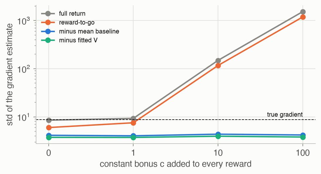
This page’s reach toy makes the point with numbers. A point robot on a line starts at 0 and has 10 steps to reach a goal at 1; its policy moves by \(k\) times the remaining error, plus Gaussian noise of standard deviation 0.3. The reward per step is minus the squared distance to the goal, plus a constant bonus \(c\) (think of a reward for every step the robot stays upright). The bonus changes nothing about which gain is best, \(k = 1\). It does change the noise. From batches of 16 episodes at \(k =\) 0.3, the true gradient is 8.78. With \(c = 0\) the four estimators of Figure 3 have standard deviations 8.53, 5.99, 4.14, 3.75: each fix helps. With \(c = 100\) the full-return estimator’s spread grows to 1,530, so the signal is 0.6% of the noise, while the estimators with a baseline stay at 4.20 and 3.81.
The advantage
Look at what the reward-to-go estimates: the expected sum of future rewards after taking \(a_t\) in \(s_t\) and following the policy, which is exactly \(Q^\pi(s_t, a_t)\). The reward-to-go is a one-sample, noisy estimate of Q ▶ 22:14. The natural baseline for a state is what the policy expects there on average, \(V^\pi(s_t)\). Their difference is the advantage: positive if the action did better than usual from this state, negative if worse ▶ 22:47. A state-dependent baseline accounts for how hard each state is; in the reach toy, a value function fitted on a separate batch beats the mean baseline (3.75 against 4.14).
Reusing data: importance sampling
Every estimate so far assumes the samples came from the current policy. After one gradient step the policy has changed, so the batch must be thrown away and a new one collected. For a real robot, where every episode costs time and wear, that is wasteful ▶ 24:53. Importance sampling estimates an expectation under one distribution using samples from another, by weighting each sample by the ratio of the two probabilities ▶ 25:54. Two caveats. The old policy must give nonzero probability wherever the new one does, or the ratio is undefined; and the estimate is only reliable while the two distributions are close ▶ 27:28.
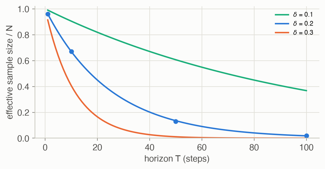
For whole trajectories the dynamics cancel again, leaving a product of per-step ratios ▶ 28:30. Products of many factors explode or vanish: the variance grows exponentially with the horizon ▶ 30:03. If each step’s ratio compares two Gaussians whose means differ by 0.2 standard deviations, the trajectory weight’s effective sample size is 67% of the batch after 10 steps and 1.8% after 100 (Figure 4). So in practice each time step is reweighted by its own action ratio only, ignoring how the state distribution changed; TRPO and PPO justify that approximation by keeping updates small ▶ 31:36. With it, one batch can serve several gradient steps ▶ 32:37.
How far may one batch move the policy?
If the new policy puts probability on actions the old policy never took, the ratio is meaningless. An entropy bonus in the objective keeps the policy spread out, so that its support does not collapse ▶ 33:40. If the policy moves too far within one batch, ratios explode: an action the old policy took with probability 0.005 that the new policy takes with probability 0.10 gets weight 20 ▶ 35:45. TRPO maximizes the reweighted advantage subject to a bound on the KL divergence between old and new policies ▶ 36:46. It comes with a guarantee that each update does not make the policy worse, but the constraint needs second-order information about the KL divergence, which is expensive for large networks ▶ 37:50. PPO gets most of the stability with a first-order trick: clip the ratio to \([1 - \epsilon, 1 + \epsilon]\) inside the objective, and take the minimum with the unclipped term ▶ 40:29. It works with ordinary optimizers such as Adam, which is why it also trains large language models (RLHF, GRPO); it gives up the guarantee and still needs many fresh samples ▶ 41:02.
The reuse toy measures what clipping buys. A one-step task with a continuous action: a Gaussian policy starting at \(\mathcal{N}(0, 1)\), and a reward bump at \(a = 2\), observed with noise. Each run collects 30 batches of 32 samples and takes \(K\) gradient steps on each batch, over 50 seeds. One step per batch, the on-policy method, reaches an average expected reward of only 0.19 (the best possible is 1). Reuse helps a lot: with \(K = 10\) clipped steps per batch it reaches 0.96. Without the clip, more reuse becomes harmful. At \(K = 20\), 20% of the runs lose the bump entirely (expected reward below 0.05), and 44% at \(K = 100\); with the clip, none do at any \(K\) (Figure 5).
What to watch for. In the first batch the samples spread from -2.3 to 1.4, none near the top of the bump. Far from the bump every reward is just noise, so blue and orange dots are mixed: off the bump, only 38% of the first ten batches’ samples are blue. The few samples that land on the bump’s slope are blue 89% of the time, and they do the pulling: the curve drifts right, and it even widens slightly, to a standard deviation of 1.27 at batch 3, since spreading out reaches more of the bump. From batch 12 the curve covers the bump and narrows. In the last ten batches every sample lands on the bump and blue sits above orange: which samples beat the average is now mostly noise (52% are blue), the pulls largely cancel, and the mean moves 0.026 per batch, against 0.123 in the first ten. After 30 batches the policy has standard deviation 0.15, is centred at 1.99, and the counter’s expected reward has risen from 0.09 to 0.96.
Actor and critic
PPO’s full objective has three terms: the clipped policy objective, a squared error that trains a value function, and the entropy bonus ▶ 43:05. The policy is the actor; the value function, which supplies the advantages, is the critic. Together they form an actor-critic: direct optimization of the behavior you care about, with a learned baseline to keep the variance low ▶ 44:37. The critic learns by temporal-difference updates, bootstrapping from its own next-state estimate instead of waiting for the episode to end: more sample-efficient, at the cost of a small bias ▶ 45:39. Since the critic is only needed during training, in simulation it can be given privileged information, such as exact object poses, that the deployed policy never sees ▶ 46:09.
The lecture’s robot examples: quadruped locomotion over rough terrain trained with TRPO in simulation and transferred to the real robot ▶ 39:25, and OpenAI’s Rubik’s-cube hand, 24 degrees of freedom, trained with PPO and heavy randomization of the simulator, with the cube’s pose estimated by a separate vision network ▶ 42:05.
Fully off-policy: SAC
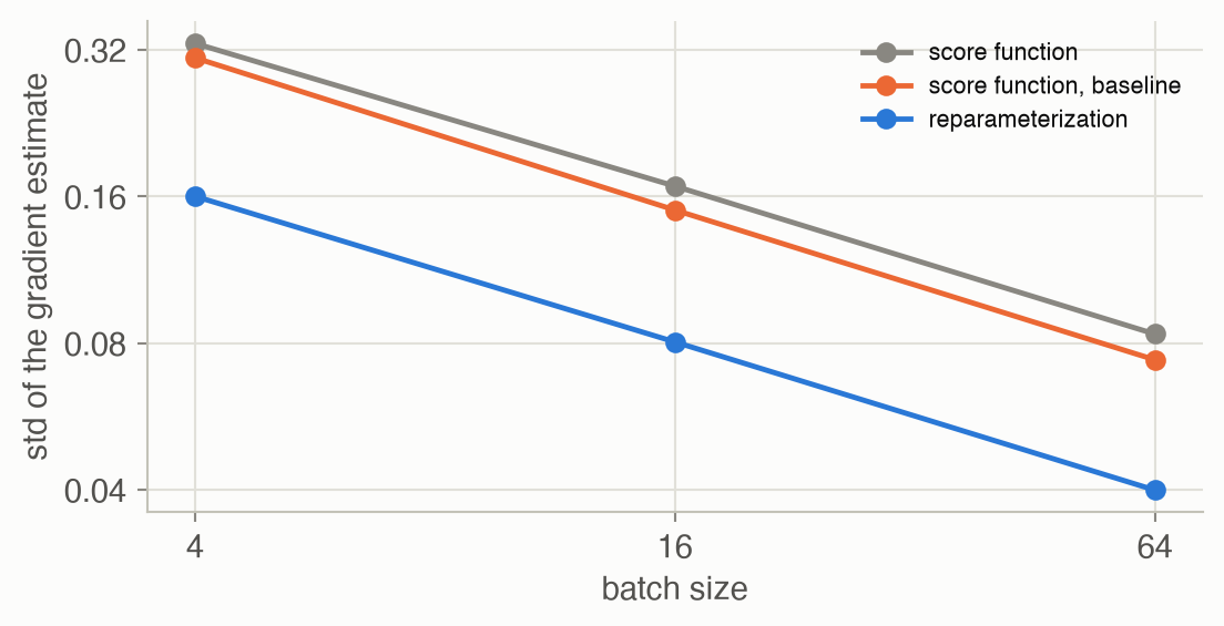
Soft actor-critic closes the lecture’s arc from on-policy to off-policy. Its critic is a Q-function trained by TD updates on a replay buffer, as in DQN ▶ 47:13. Its actor maximizes the critic’s score plus an entropy bonus; the bonus also enters the critic’s target, which favours states with many good ways to proceed ▶ 48:16. The key move is that the actor takes old states from the buffer but asks the current policy what it would do there, and lets the critic estimate how good that new action is: the critic acts as a learned simulator ▶ 48:47. To pass the critic’s gradient back through the sampled action, SAC writes the sample as \(a = \mu_\theta(s) + \sigma_\theta(s)\,\varepsilon\) with fixed noise \(\varepsilon\): the reparameterization trick ▶ 49:17. In this page’s third toy, that pathwise gradient has 0.48 times the standard deviation of the score-function gradient for the same samples (Figure 6).
Key concepts & formulae
The lecture’s notation: \(\pi_\theta(a \mid s)\) for the policy, \(p_\theta(\tau)\) for the distribution over trajectories \(\tau = (s_0, a_0, s_1, \dots)\), \(R(\tau)\) for a trajectory’s return and \(J(\theta)\) for the expected return; \(\theta'\) is the new policy, \(\theta\) the one that collected the data. The ADM book writes \(U(\theta)\) for \(J(\theta)\) and calls PPO’s clipped objective the clamped surrogate.
The policy gradient
\[ \begin{aligned} J(\theta) &= \mathbb{E}_{\tau \sim p_\theta(\tau)}\big[R(\tau)\big] \\ p_\theta(\tau) &= p(s_0) \textstyle\prod_{t} \pi_\theta(a_t \mid s_t)\, P(s_{t+1} \mid s_t, a_t) \end{aligned} \tag{1}\]
In words. A policy is as good as the average return of the trajectories it produces. A trajectory’s probability is the start-state probability times, at every step, the policy’s probability of its action and the world’s probability of the next state.
Term by term.
- \(R(\tau) = \sum_t \gamma^t r_t\): the (discounted) return of one trajectory, as in Week 2.
- \(\pi_\theta\): the only factor we control. \(p(s_0)\) and \(P\) are the world’s, unknown to us.
- The lecture estimates \(J\) by averaging the returns of \(N\) rollouts ▶ 04:37.
\[ \nabla_\theta p_\theta(\tau) = p_\theta(\tau)\, \nabla_\theta \log p_\theta(\tau) \tag{2}\]
In words. The gradient of a probability equals the probability times the gradient of its logarithm.
Term by term.
- It is the chain rule, \(\nabla \log p = \nabla p / p\), rearranged.
- Its use: in \(\nabla J = \int \nabla_\theta p_\theta(\tau) R(\tau)\, d\tau\) the integrand is not a probability times something, so samples cannot estimate it. After the trick it is \(p_\theta(\tau)\) times something, which is an expectation ▶ 09:15.
\[ \nabla_\theta J(\theta) = \mathbb{E}_{\tau \sim p_\theta}\Big[\textstyle\sum_{t} \nabla_\theta \log \pi_\theta(a_t \mid s_t)\; R(\tau)\Big] \tag{3}\]
In words. To find which way to move \(\theta\), take each sampled trajectory, ask which direction makes its actions more likely, and weight that direction by the trajectory’s return. Average over trajectories.
Term by term.
- \(\nabla_\theta \log \pi_\theta(a_t \mid s_t)\): the score of one action. For a Gaussian policy with mean \(\mu_\theta(s)\) and standard deviation \(\sigma\) it is \(\frac{a_t - \mu_\theta(s_t)}{\sigma^2}\, \nabla_\theta \mu_\theta(s_t)\): the noise that was drawn, times how \(\theta\) moves the mean.
- \(R(\tau)\): the weight. With \(R \equiv 1\) this would be behavior cloning on the robot’s own actions ▶ 14:58.
- No \(P(s_{t+1} \mid s_t, a_t)\) appears: the method is model-free.
Why it holds. Apply Equation 2 to \(\nabla J = \int \nabla_\theta p_\theta(\tau) R(\tau)\, d\tau\) to get \(\mathbb{E}[\nabla_\theta \log p_\theta(\tau)\, R(\tau)]\). By Equation 1, \(\log p_\theta(\tau) = \log p(s_0) + \sum_t \log \pi_\theta(a_t \mid s_t) + \sum_t \log P(s_{t+1} \mid s_t, a_t)\); the first and last terms do not depend on \(\theta\), so their gradients vanish ▶ 12:55.
Numeric check. In the reach toy at \(k =\) 0.3, the average of Equation 3 over many batches of 16 is 8.91, against a true gradient of 8.78 (from 2 million episodes).
Less variance, same gradient
\[ \nabla_\theta J(\theta) = \mathbb{E}\Big[\textstyle\sum_{t} \nabla_\theta \log \pi_\theta(a_t \mid s_t) \big(\textstyle\sum_{t' \ge t} r_{t'} - b\big)\Big] \tag{4}\]
In words. Weight each action by the rewards that came after it, minus a baseline. The expected gradient is the same as in Equation 3; the noise is lower.
Term by term.
- \(\sum_{t' \ge t} r_{t'}\): the reward-to-go. Rewards before \(t\) are dropped: on average they contribute nothing, because the action at \(t\) cannot have caused them ▶ 17:03.
- \(b\): the baseline, for example the batch’s average return ▶ 19:40. It may depend on the state, but not on the action.
Why it holds. For any \(b\) that does not depend on \(a_t\): \(\mathbb{E}_{a \sim \pi_\theta}[\nabla_\theta \log \pi_\theta(a \mid s)\, b] = b \int \nabla_\theta \pi_\theta(a \mid s)\, da = b\, \nabla_\theta \int \pi_\theta(a \mid s)\, da = b\, \nabla_\theta 1 = 0\). The same argument removes past rewards, which are fixed by the time \(a_t\) is drawn.
Numeric check. A baseline must not use the episode it is subtracted from: the reach toy’s first version used the batch mean including the episode itself and a value function fitted on the same batch, and both estimates came out biased. The page’s version uses the mean of the other episodes and a value function fitted on a separate batch; all four averages agree with the true gradient within four standard errors, at every offset \(c\).
\[ \begin{aligned} A^\pi(s, a) &= Q^\pi(s, a) - V^\pi(s) \\ \nabla_\theta J(\theta) &= \mathbb{E}\Big[\textstyle\sum_{t} \nabla_\theta \log \pi_\theta(a_t \mid s_t)\; A^\pi(s_t, a_t)\Big] \end{aligned} \tag{5}\]
In words. How much better taking \(a\) in \(s\) is than what the policy does on average there. Using it as the weight pushes up better-than-usual actions and pushes down worse-than-usual ones.
Term by term.
- \(Q^\pi(s_t, a_t)\): the expected reward-to-go; the observed reward-to-go is one noisy sample of it ▶ 22:14.
- \(V^\pi(s) = \mathbb{E}_{a \sim \pi}[Q^\pi(s, a)]\): the state-dependent baseline. In practice a learned critic estimates it.
- \(\mathbb{E}_{a \sim \pi}[A^\pi(s, a)] = 0\): on average, the policy is exactly as good as itself.
Reusing data
\[ \mathbb{E}_{x \sim p}\big[f(x)\big] = \mathbb{E}_{x \sim q}\Big[\frac{p(x)}{q(x)}\, f(x)\Big] \tag{6}\]
In words. An average under \(p\) can be computed from samples of \(q\), if each sample is weighted by how much more (or less) likely it is under \(p\) than under \(q\).
Term by term.
- \(p\): the new policy’s distribution, the one we want to evaluate; \(q\): the old policy’s, which produced the data.
- \(p(x)/q(x)\): the importance weight. Its average under \(q\) is 1.
- Requires \(q(x) > 0\) wherever \(p(x) > 0\); otherwise the weight is undefined ▶ 27:28.
Why it holds. Multiply and divide by \(q(x)\) inside the integral: \(\int p(x) f(x)\, dx = \int q(x) \frac{p(x)}{q(x)} f(x)\, dx\), the same “multiply by one” step as Equation 2.
\[ \nabla_{\theta'} J(\theta') \approx \mathbb{E}_{(s_t, a_t) \sim \pi_\theta}\Big[\frac{\pi_{\theta'}(a_t \mid s_t)}{\pi_\theta(a_t \mid s_t)}\; \nabla_{\theta'} \log \pi_{\theta'}(a_t \mid s_t)\; A^{\pi_\theta}(s_t, a_t)\Big] \tag{7}\]
In words. Reuse the old policy’s samples for the new policy’s gradient, weighting each step by its own action ratio.
Term by term.
- The exact weight for a whole trajectory is \(\prod_t \pi_{\theta'}(a_t \mid s_t) / \pi_\theta(a_t \mid s_t)\), whose variance grows exponentially with the horizon (Figure 4).
- The per-step version also needs the ratio of state distributions under the two policies, which would require the dynamics; it is approximated by 1 ▶ 31:36. That is accurate only while \(\theta'\) stays near \(\theta\).
- At \(\theta' = \theta\) the ratio is 1 and this is Equation 5.
Numeric check. When each step’s two Gaussians have means \(\delta\) standard deviations apart, each ratio has \(\mathbb{E}[w^2] = e^{\delta^2}\), so the trajectory weight has \(\mathbb{E}[w^2] = e^{T\delta^2}\) and an effective sample size of \(e^{-T\delta^2}\) of the batch. For \(\delta = 0.2\) and \(T = 50\) that is 0.135; sampled weights give 0.130.
Keeping the policy close
\[ \begin{aligned} L(\theta') &= L_{\text{PG}}(\theta') + \beta\, \mathcal{H}\big(\pi_{\theta'}(\cdot \mid s)\big) \\ \mathcal{H}_{\text{Gauss}} &= \tfrac{d}{2}\big(1 + \log 2\pi\big) + \textstyle\sum_{i=1}^{d} \log \sigma_i \end{aligned} \tag{8}\]
In words. Reward the policy for staying spread out, so it keeps giving some probability to actions it is not currently favouring.
Term by term.
- \(\beta\): the temperature; larger means more spread, near 0 means greedy ▶ 34:11.
- For discrete actions, \(\mathcal{H} = -\sum_a \pi(a) \log \pi(a)\) (Shannon entropy); for a Gaussian over \(d\) action dimensions, the second line, which depends only on the standard deviations ▶ 34:43.
- With a Gaussian over an unbounded action space, the bonus grows without limit as \(\sigma\) grows, so a large \(\beta\) can make the policy ever wider. SAC squashes its actions into a bounded range with \(\tanh\), which keeps the entropy bounded.
\[ \begin{aligned} \max_{\theta'}\; & \mathbb{E}_{s, a \sim \pi_\theta}\Big[\frac{\pi_{\theta'}(a \mid s)}{\pi_\theta(a \mid s)}\, A^{\pi_\theta}(s, a)\Big] \\ \text{subject to}\; & \mathbb{E}_{s}\big[D_{\text{KL}}\big(\pi_\theta(\cdot \mid s) \,\big\|\, \pi_{\theta'}(\cdot \mid s)\big)\big] \le \delta \end{aligned} \tag{9}\]
In words. Improve the reweighted advantage as much as possible, but never let the new policy’s action distribution move further than \(\delta\) from the old one, measured by KL divergence.
Term by term.
- The objective is the off-policy surrogate whose gradient is Equation 7.
- \(D_{\text{KL}}\): how different two distributions are; it is zero only when they are equal, and it becomes very large if the new policy gives almost no probability to actions the old one took.
- \(\delta\): the trust-region size. Solving the constrained problem needs the Fisher information matrix (second derivatives of the KL), whose size is the number of parameters squared; TRPO approximates it with conjugate gradients ▶ 38:23.
\[ \begin{aligned} \rho &= \pi_{\theta'}(a \mid s) / \pi_\theta(a \mid s) \\ L^{\text{CLIP}}(\theta') &= \mathbb{E}\big[\min\big(\rho A,\; \operatorname{clip}(\rho, 1 - \epsilon, 1 + \epsilon)\, A\big)\big] \end{aligned} \tag{10}\]
In words. Use the reweighted advantage, but stop rewarding a sample once its ratio has moved more than \(\epsilon\) in the direction its advantage favours.
Term by term.
- \(A\): the advantage \(A^{\pi_\theta}(s, a)\), from the critic.
- \(A > 0\): the term grows with \(\rho\) only up to \(1 + \epsilon\); beyond that its gradient is zero. \(A < 0\): likewise below \(1 - \epsilon\).
- The \(\min\) keeps the unclipped term when it is lower: a sample whose ratio moved the wrong way (an action with \(A > 0\) that became less likely) still pulls the policy back. The objective is a pessimistic bound.
- \(\epsilon\): typically 0.1–0.3; the reuse toy uses 0.2.
Numeric check. On the explorer’s batch (seed 0, first batch of the reuse toy), the clipped objective is largest at \(\mu' =\) 0.10, \(\sigma' =\) 1.25, close to the old policy \(\mathcal{N}(0, 1)\). The unclipped objective has no maximum at all: it keeps growing as the new policy shrinks onto the batch’s single best sample, at \(a =\) 1.37. On a grid it peaks at the grid’s edge, \(\sigma' = 0.02\) (Figure 9).
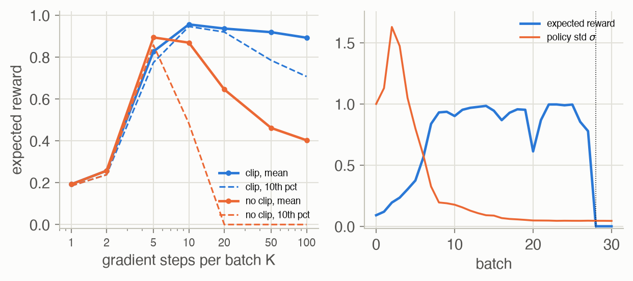
The right panel shows how an unclipped run fails. The policy first widens while it searches, then finds the bump and narrows. Without the clip it keeps narrowing: after 20 batches with \(K = 20\), the median standard deviation over the 50 seeds is 0.052 without the clip and 0.147 with it. In this run it is 0.046 at batch 28. The gradient with respect to the mean scales as \(1/\sigma^2\), so a few lucky samples in that batch move the mean by 43 standard deviations. Afterwards every sample in the batch has a ratio near zero (the largest is below \(10^{-3}\)): the new policy has left the data’s support, landed where the reward is flat, and never comes back.
\[ L^{\text{PPO}}(\theta') = \mathbb{E}\big[L^{\text{CLIP}}(\theta') - c_1 \big(V_{\theta'}(s) - V^{\text{targ}}\big)^2 + c_2\, \mathcal{H}(\pi_{\theta'})(s)\big] \tag{11}\]
In words. Maximize the clipped objective, train the value function towards its targets, and keep the policy spread out, all in one loss.
Term by term.
- \(L^{\text{CLIP}}\): the actor’s term, Equation 10.
- \((V_{\theta'}(s) - V^{\text{targ}})^2\): the critic’s regression loss, with a minus sign because the whole objective is maximized; the critic supplies the advantages ▶ 43:36.
- \(c_1\), \(c_2\): weights of the critic loss and the entropy bonus (Equation 8).
Soft actor-critic
\[ \begin{aligned} L_{\text{actor}}(\theta) &= \mathbb{E}_{s \sim \mathcal{D},\, a \sim \pi_\theta}\big[\alpha \log \pi_\theta(a \mid s) - Q_\phi(s, a)\big] \\ y &= r + \gamma\, \mathbb{E}_{a' \sim \pi_\theta}\big[Q_{\bar\phi}(s', a') - \alpha \log \pi_\theta(a' \mid s')\big] \\ L_{\text{critic}}(\phi) &= \mathbb{E}_{(s, a, r, s') \sim \mathcal{D}}\big[(Q_\phi(s, a) - y)^2\big] \end{aligned} \tag{12}\]
In words. The actor picks actions the critic scores highly while staying random (high entropy). The critic regresses on a TD target that includes the entropy of the next action.
Term by term.
- \(\mathcal{D}\): the replay buffer; states and transitions come from any past policy, so both losses are off-policy.
- \(a \sim \pi_\theta\) in the actor loss: the current policy’s action in an old state, scored by the critic ▶ 48:47.
- \(\alpha \log \pi_\theta\): minus the entropy, weighted by the temperature \(\alpha\) (the lecture’s \(\beta\) in Equation 8).
- \(Q_{\bar\phi}\): a slowly updated target copy of the critic, as in DQN.
\[ \begin{aligned} a &= \mu_\theta(s) + \sigma_\theta(s)\, \varepsilon, \qquad \varepsilon \sim \mathcal{N}(0, 1) \\ \nabla_\theta\, \mathbb{E}_a\big[Q(s, a)\big] &= \mathbb{E}_\varepsilon\big[\nabla_a Q(s, a)\; \nabla_\theta a\big] \end{aligned} \tag{13}\]
In words. Write the random action as a deterministic function of the parameters and of noise that does not depend on them. Then the gradient can pass through the action into the critic, by the chain rule.
Term by term.
- \(\varepsilon\): drawn from a fixed distribution with no parameters, so nothing about the sampling needs a gradient ▶ 49:17.
- \(\nabla_a Q\): the critic’s slope in the action, as in DDPG’s actor update (Week 4). The score-function estimator (Equation 3) does not need it; the pathwise estimator does.
- Both are unbiased; the pathwise estimator is usually far less noisy.
Numeric check. For \(a \sim \mathcal{N}(0.5, 0.5^2)\) and the reward bump as \(Q\), the exact \(\partial_\mu \mathbb{E}[Q]\) is 0.2236. With 16 samples, the score-function estimate has standard deviation 0.168, 0.150 with a baseline, and the reparameterized one 0.080; all three average to the exact value.
Worked examples
Example 1: one batch, four estimators
Four episodes of the reach task at \(k =\) 0.3 with the bonus \(c = 10\), so each episode’s return is near 100. Each row is one episode: its return, and what it contributes to the gradient estimate under three of the weightings (the estimate is the average of a column).
| episode | return | full return | reward-to-go | minus mean baseline |
|---|---|---|---|---|
| 1 | 98.4 | +453.9 | +273.0 | +2.6 |
| 2 | 98.9 | +655.4 | +600.1 | +5.8 |
| 3 | 96.5 | -386.2 | -486.0 | +17.7 |
| 4 | 98.7 | +595.1 | +540.5 | +5.1 |
| average | +329.6 | +231.9 | +7.8 |
The returns differ by only a few units, but the full-return column is dominated by the shared bonus: each entry is the episode’s summed score, a random number around zero, multiplied by a number near 100. The reward-to-go column multiplies later scores by smaller numbers, because fewer rewards remain, but still carries the bonus. Subtracting the other episodes’ mean reward-to-go at each step removes it, leaving entries of the size of the true gradient, 8.8.
Example 2: clipping, sample by sample
Five samples from the explorer’s batch (old policy \(\mathcal{N}(0, 1)\)), evaluated for a new policy that has moved its mean to 0.6 with \(\epsilon = 0.2\):
| action a | advantage A | ratio ρ | ρA | clipped term | gradient |
|---|---|---|---|---|---|
| -1.01 | +0.398 | 0.46 | +0.181 | +0.181 | still pushes |
| -0.46 | -0.255 | 0.63 | -0.162 | -0.204 | switched off |
| +0.10 | -0.017 | 0.89 | -0.015 | -0.015 | still pushes |
| +0.95 | +0.433 | 1.47 | +0.638 | +0.519 | switched off |
| +1.37 | +0.521 | 1.90 | +0.988 | +0.625 | switched off |
Moving the mean right raises the ratios of actions on the right and lowers those on the left. A sample is switched off when its ratio has already moved past \(1 \pm 0.2\) in the direction its advantage asked for: a right-hand action with \(A > 0\) and \(\rho > 1.2\), or a left-hand one with \(A < 0\) and \(\rho < 0.8\). Its gradient is then zero, so further steps on this batch are driven only by the remaining samples. A sample whose ratio moved the other way keeps its unclipped term, which is the smaller of the two, and pulls the policy back.
Example 3: the 99-and-101 reaches, with numbers
Two episodes with returns 99 (overshoot) and 101 (perfect), and suppose the summed scores of their actions are \(g_1 = +0.5\) and \(g_2 = -0.3\) (random numbers, as they would be). REINFORCE’s estimate is \(\frac{1}{2}(99 \times 0.5 + 101 \times (-0.3)) = 9.6\): dominated by the large common return, with the first, worse episode’s direction winning. With baseline \(b = 100\): \(\frac{1}{2}((-1) \times 0.5 + 1 \times (-0.3)) = -0.4\). The weights now reflect that episode 2 was better: its direction is followed, episode 1’s is reversed. On average over many episodes both estimates agree; in any one batch the first is mostly noise.
Interactive
Gradient noise, with and without baselines
What to try. At \(c = 0\) the four histograms are centred on the same value and differ only in width. Move to \(c = 10\) and \(c = 100\): the top two spread over hundreds and then thousands (look at their axes), while the bottom two do not change at all. In a single batch at \(c = 100\), the full-return estimate is as likely to point the wrong way as the right way; that is what it means for the signal to be 0.6% of the noise.
PPO’s clip, on one batch
The 32 samples are the first batch of the reuse toy, drawn from the old policy \(\mathcal{N}(0, 1)\); the dots sit at their advantages. Move the new policy and watch which samples still push it (filled) and which the clip has switched off (hollow).
What to try. Start at the old policy (\(\mu' = 0\), \(\sigma' = 1\)): every ratio is 1, both objectives are 0, and every dot is filled. Move \(\mu'\) right: the unclipped objective rises, and samples on the right with positive advantage start to switch off once their ratios pass \(1 + \epsilon\). Now shrink \(\sigma'\) towards 0.05 with \(\mu'\) near 1.37, where the batch’s best sample sits. The unclipped objective keeps climbing, because the ratio of that one sample grows without limit. The true change in expected reward does not follow it, since the bump is at 2, not at that sample. The clipped objective flattens out instead: it cannot be raised much by any single sample. A larger \(\epsilon\) lets the policy move further before samples switch off.
Reuse, step by step
What to try. At \(K = 1\) the two curves are the same, since a single step from the old policy has ratio 1 and nothing to clip, and learning is slow. Increase \(K\): each batch now buys more progress, and up to \(K = 5\) the clip barely matters (unclipped is even slightly faster). From \(K = 20\) the orange band reaches down to 0: some unclipped runs fit one batch’s noise so hard that they leave the bump for good. The blue band stays narrow. The clip turns \(K\) from a dangerous knob into a forgiving one.
Algorithm & code
The course’s homework asks students to implement PPO (its clipped objective, value loss, entropy term and KL check) and SAC (its critic target, actor and temperature losses, and target-network update), so this page shows equations and results for those, not code. The code below covers the rest of the lecture: the REINFORCE estimators, with reward-to-go and baselines, and the reparameterization trick.
REINFORCE: four weightings of the same score
def reach_rollouts(k, n, rng, c=0.0) -> tuple[Array, Array, Array]:
    """n episodes from x_0 = 0 with gain k; reward c - (x_{t+1} - g)^2 per step.

    Returns the errors e_t = g - x_t, the score d/dk log pi(a_t | x_t),
    and the rewards, each of shape (n, T).
    """
    x = np.zeros(n)
    e, a, r = (np.empty((n, T)) for _ in range(3))
    for t in range(T):
        e[:, t] = GOAL - x
        a[:, t] = k * e[:, t] + SIGMA * rng.standard_normal(n)
        x = x + a[:, t]
        r[:, t] = c - (x - GOAL) ** 2
    # log N(a; k e, sigma^2) = -(a - k e)^2 / (2 sigma^2) + const, so its
    # derivative in k is (a - k e) e / sigma^2: noise times state, scaled.
    score = (a - k * e) * e / SIGMA**2
    return e, score, r

def reward_to_go(r) -> Array:
    """sum_{t' >= t} r_t' for every t: a reversed cumulative sum, (n, T)."""
    return np.cumsum(r[:, ::-1], axis=1)[:, ::-1]

def fit_value(e, rtg) -> Array:
    """Per-step least squares V_t(e) = w0 + w1 e^2; returns weights (T, 2)."""
    w = []
    for t in range(T):
        X = np.stack([np.ones(len(e)), e[:, t] ** 2], axis=1)   # (n, 2)
        w.append(np.linalg.lstsq(X, rtg[:, t], rcond=None)[0])
    return np.array(w)

def gradient_estimates(k, n, rng, c=0.0) -> dict[str, float]:
    """One batch of n episodes, four estimates of dJ/dk (same samples)."""
    e, score, r = reach_rollouts(k, n, rng, c)
    rtg = reward_to_go(r)
    # A baseline must not depend on the episode it is subtracted from, or it
    # biases the estimate: use the mean of the *other* n - 1 episodes, and
    # fit V on a separate batch, as a critic trained on earlier data would be.
    loo_mean = (rtg.sum(0) - rtg) / (n - 1)
    e_fit, _, r_fit = reach_rollouts(k, n, rng, c)
    w = fit_value(e_fit, reward_to_go(r_fit))     # (T, 2)
    V = w[:, 0] + w[:, 1] * e**2                  # (n, T), broadcast over n
    weights = (r.sum(1, keepdims=True), rtg, rtg - loo_mean, rtg - V)
    return {name: float((score * wt).sum(1).mean())
            for name, wt in zip(ESTIMATORS, weights)}
import torch
import torch.nn as nn
from rlc.toys import w05_pg as reach # the reach task on this page
torch.manual_seed(0)
T, G = reach.T, reach.GOAL
# Policy: mean = k * error, with a learned log std (starts at sigma = 0.3).
policy = nn.Linear(1, 1, bias=False)
nn.init.zeros_(policy.weight) # k = 0: does not move
log_std = nn.Parameter(torch.tensor(-1.2))
# Critic: V(t / T, error), a small MLP used only as a baseline.
value = nn.Sequential(nn.Linear(2, 32), nn.Tanh(), nn.Linear(32, 1))
opt_pi = torch.optim.Adam([*policy.parameters(), log_std], lr=0.02)
opt_v = torch.optim.Adam(value.parameters(), lr=0.01)
def rollout(n):
"""n episodes in parallel. Returns log-probs (n, T),
critic features (n, T, 2) and rewards (n, T)."""
x = torch.zeros(n, 1)
logps, feats, rewards = [], [], []
for t in range(T):
e = G - x # (n, 1)
dist = torch.distributions.Normal(policy(e), log_std.exp())
# sample() cuts the graph: gradients reach theta via log_prob only
a = dist.sample()
logps.append(dist.log_prob(a).squeeze(-1))
feats.append(torch.cat([torch.full_like(e, t / T), e], dim=-1))
x = x + a
rewards.append((-(x - G) ** 2).squeeze(-1))
return (torch.stack(logps, 1), torch.stack(feats, 1),
torch.stack(rewards, 1))
for it in range(500):
logp, feat, r = rollout(64)
rtg = r.flip(1).cumsum(1).flip(1) # reward-to-go, (64, T)
v = value(feat).squeeze(-1) # (64, T)
# Advantage = reward-to-go minus the critic's baseline. detach(): the
# policy loss must not push gradients into the critic.
adv = (rtg - v).detach()
loss_pi = -(logp * adv).sum(1).mean() # minimize minus eq. rtg
loss_v = ((v - rtg) ** 2).mean() # critic: fit the returns
opt_pi.zero_grad(); loss_pi.backward(); opt_pi.step()
opt_v.zero_grad(); loss_v.backward(); opt_v.step()
k = policy.weight.item()
assert 0.85 < k < 1.15, k # learned the best gain, 1The four NumPy estimators differ only in the weight multiplied onto the same score; the PyTorch sketch uses the last one, with the baseline learned by a small critic network. Written as a loss, the policy gradient is “log-probability times a detached weight”, which automatic differentiation turns into Equation 4.
The reparameterization trick
def mu_gradient_estimates(mu, sigma, n, rng) -> dict[str, float]:
    """Three unbiased estimates of d/dmu E[bump(a)] from one batch of n."""
    eps = rng.standard_normal(n)
    a = mu + sigma * eps
    q = bump(a)
    # d/dmu log N(a; mu, sigma^2) = (a - mu) / sigma^2 = eps / sigma
    score = eps / sigma
    loo = (q.sum() - q) / (n - 1) if n > 1 else 0.0     # leave-one-out baseline
    return {"score function": float((q * score).mean()),
            "score function, baseline": float(((q - loo) * score).mean()),
            # a = mu + sigma * eps, so da/dmu = 1 and the gradient is Q'(a)
            "reparameterization": float(bump_slope(a).mean())}
from torch.distributions import Normal
def q(a):
"""Stand-in critic: the page's reward bump, in torch."""
return torch.exp(-0.5 * ((a - reach.BUMP_AT) / reach.BUMP_WIDTH) ** 2)
def per_batch_grads(reparam, B=4000, n=16):
"""B independent estimates of d/dmu E[q(a)], a ~ N(0.5, 0.5^2).
Each batch gets its own copy of mu, shape (B, 1), so one backward pass
of the summed loss leaves batch i's gradient in mu.grad[i]."""
mu = torch.full((B, 1), 0.5, requires_grad=True)
dist = Normal(mu.expand(B, n), 0.5)
if reparam:
a = dist.rsample() # mu + 0.5 * eps: graph kept
loss = q(a).mean(1).sum()
else:
a = dist.sample() # no graph: use log_prob
loss = (q(a) * dist.log_prob(a)).mean(1).sum()
loss.backward()
return mu.grad.squeeze(1) # (B,)
g_sf, g_rp = per_batch_grads(False), per_batch_grads(True)
exact = reach.mu_gradient_exact(0.5, 0.5)
assert abs(g_sf.mean() - exact) < 0.02 and abs(g_rp.mean() - exact) < 0.02
assert g_rp.std() < 0.6 * g_sf.std() # same mean, much less noisesample() returns a number with no history, so the score-function estimator must go through log_prob; rsample() builds the sample from \(\mu\), \(\sigma\) and fixed noise, so the critic’s slope flows back to \(\mu\). SAC’s actor loss (Equation 12) is computed on rsample() actions for exactly this reason.
Papers
Papers discussed in class
Key papers from the lecture
Guest spotlight
Andrew Wagenmaker (UC Berkeley) argues that robots must learn from their own experience, as people do when they learn to iron a shirt: watch a video, then try, see what happens, and adjust ▶ 01:33. Each of today’s data sources falls short on its own: simulators struggle with cloth, internet video has no motor commands, and human demonstrations are expensive and still leave a gap between demonstration and deployment ▶ 03:35. The central difficulty of learning from experience, in his view, is exploration: collecting the experience that tells correct behavior apart from incorrect behavior ▶ 05:09. The textbook picture, an agent taking random actions until it stumbles on reward, does not scale to the physical world; a person exploring tries a handful of sensible options, such as picking up the iron, the shirt or the spray bottle ▶ 08:46.
His first idea gets that structured exploration from a behavior-cloning policy. A diffusion or flow policy maps Gaussian noise to an action that looks like a demonstration, so different noise inputs give different reasonable actions ▶ 11:21. Instead of exploring in action space, explore in the noise space: keep the trained policy fixed, and learn with RL a small noise policy, and a critic over noise, that choose which noise to feed it ▶ 13:57. This is DSRL (Diffusion Steering via RL, a Week 6 paper). On a real pick-and-place task its attempts looked purposeful from the start, while an action-space RL baseline flailed in free space; after 25 episodes it had locked onto the correct behavior ▶ 18:35. It also sidesteps the problem that diffusion policies have no tractable likelihood, which standard policy gradients need ▶ 19:06. He reports policies going from below 50% to 90–100% success in 30 to 90 minutes of online training ▶ 19:36.
His second idea asks whether behavior cloning is the right pre-training for RL at all ▶ 21:40. If the demonstrations never show a needed behavior, a cloned policy never tries it, and RL fine-tuning has nothing to reinforce ▶ 22:42. Adding random noise to the cloned policy trades performance against exploration ▶ 24:16. His answer is to model the uncertainty about what the demonstrator would do, and to explore more where demonstrations are scarce and less where they agree ▶ 25:18; the paper is Posterior Behavioral Cloning (arXiv 2512.16911). On a pick-and-place task both pre-trained policies started out similar, but online RL took the standard one to below 50% and his to 75% ▶ 26:20.
How it connects to this week. Both ideas are about the support problem that the lecture’s entropy bonus addresses: RL can only improve on actions the policy actually tries. Steering in noise space keeps every action inside what the demonstrations made plausible, while a posterior BC policy widens the support exactly where the data are uncertain. In the Q&A he contrasts his approach, refining a fixed policy with a second policy, with π*0.6’s advantage-conditioned training of one policy (a Week 9 paper), and says it is not yet understood when each is better ▶ 29:25.
Solved problems
1. Why a baseline is free. For a single-step task with a Gaussian policy \(a \sim \mathcal{N}(\mu, \sigma^2)\), show directly that \(\mathbb{E}\big[\nabla_\mu \log \pi(a)\, b\big] = 0\) for any constant \(b\).
TipSolution
\(\nabla_\mu \log \pi(a) = (a - \mu)/\sigma^2\). Its expectation under \(\pi\) is \((\mathbb{E}[a] - \mu)/\sigma^2 = 0\), so multiplying by a constant \(b\) still gives 0. More generally (Equation 4), \(\mathbb{E}[\nabla \log \pi] = \int \nabla \pi = \nabla \int \pi = \nabla 1 = 0\). The baseline changes each sample’s contribution, and hence the variance, but not the average.
2. Which baseline? In the reach toy with bonus \(c = 10\), why does the fitted value function \(V_t(e)\) help a little over the mean baseline, but the mean baseline already removes almost all of the problem?
TipSolution
The bonus adds the same amount, \(c\) times the number of remaining steps, to every episode’s reward-to-go at step \(t\). Any baseline that tracks the average reward-to-go per step removes it entirely; the mean of the other episodes does. What remains is the variation between episodes at the same step, which comes from how far each robot still is from the goal. The fitted value function predicts that from the current error \(e_t\), so it removes some of the remaining variation too: 3.96 against 4.36 here. The bonus was the big effect, and both baselines handle it.
3. A ratio, by hand. The old policy is \(\mathcal{N}(0, 1)\) and the new one \(\mathcal{N}(0.5, 1)\). What is the importance ratio for the action \(a = 1\)? For \(a = -2\)? With \(\epsilon = 0.2\) and advantages \(A = +1\) at \(a = 1\) and \(A = -1\) at \(a = -2\), which of the two samples does PPO’s clip switch off?
TipSolution
\(\rho(a) = \exp\big(-\tfrac{1}{2}(a - 0.5)^2 + \tfrac{1}{2}a^2\big) = \exp(0.5a - 0.125)\). At \(a = 1\): \(e^{0.375} \approx 1.45\). At \(a = -2\): \(e^{-1.125} \approx 0.32\). The first has \(A > 0\) and \(\rho > 1.2\): the policy already favours it beyond the trust interval, so it is switched off. The second has \(A < 0\) and \(\rho < 0.8\): the policy has already moved away from it as far as the clip allows, so it is switched off too. Both samples got what they asked for; further steps on this batch would be driven by the other samples.
4. How long can a trajectory weight be trusted? Per-step ratios have \(\mathbb{E}[w_t^2] = 1.01\) each. After how many steps has the trajectory weight’s effective sample size halved? For a 500-step episode at 50 Hz (10 seconds), what is left?
TipSolution
For independent steps \(\mathbb{E}[w^2] = 1.01^T\), and the effective sample size is \(1/1.01^T\) of the batch. It halves when \(T = \ln 2 / \ln 1.01 \approx 70\) steps. After 500 steps, \(1.01^{-500} \approx 0.007\): about 0.7% of the batch, so a batch of 1,000 trajectories behaves like 7. This is why Equation 7 keeps only the per-step ratio.
5. Score function or reparameterization? For which of these can you use the reparameterization trick: (a) a learned critic \(Q_\phi(s, a)\), (b) the real robot’s reward, measured after the action, (c) a simulator written in a differentiable physics engine?
TipSolution
The pathwise gradient (Equation 13) needs \(\nabla_a\) of whatever is being maximized. (a) Yes: the critic is a network, and SAC does exactly this. (b) No: you cannot differentiate the real world with respect to the action, so you need the score function (Equation 3), which only needs the reward’s value. (c) Yes in principle, since the simulator provides gradients, though contact-rich simulators give gradients that are often uninformative. The critic in (a) is what makes SAC’s low-variance actor update possible without a differentiable world.
Recap
- The policy gradient follows expected return without differentiating the world. The log-derivative trick turns it into an average of score-times-return, and the dynamics drop out. Why it matters: every method this week, and the RL fine-tuning of large robot policies in later weeks, starts from this estimator.
- Variance, not bias, is the practical problem. Reward-to-go and baselines leave the average gradient unchanged and shrink its noise; a constant bonus in the reward can make the plain estimator useless. Why it matters: sample cost is the binding constraint on real robots.
- The advantage is the right weight. \(A = Q - V\) asks whether an action beat the policy’s own average. Why it matters: it brings value functions back as critics, joining Week 4’s ideas with this week’s.
- Importance sampling lets a batch be reused, within limits. Per-step ratios are usable; trajectory weights are not; any reweighting fails once the policy leaves the data’s support. Why it matters: the limit explains entropy bonuses, trust regions and the clip.
- TRPO and PPO bound each update. TRPO with a KL constraint and a guarantee; PPO with a clipped ratio that is cheap and robust to how often a batch is reused. Why it matters: PPO is the default for simulated robot training and for language-model fine-tuning.
- SAC is off-policy and pathwise. A Q-critic on a replay buffer, an entropy bonus, and gradients through reparameterized actions. Why it matters: it is the most sample-efficient of the lecture’s methods, and a common choice for RL on real robots.
Cheat sheet & connections
| Name | Formula | Where |
|---|---|---|
| Objective | \(J(\theta) = \mathbb{E}_{\tau \sim p_\theta}[R(\tau)]\) | Equation 1 |
| Log-derivative trick | \(\nabla p = p\, \nabla \log p\) | Equation 2 |
| Policy gradient ★ | \(\mathbb{E}[\sum_t \nabla \log \pi\, R(\tau)]\) | Equation 3 |
| Reward-to-go, baseline | \(\sum_{t' \ge t} r_{t'} - b\) | Equation 4 |
| Advantage | \(A = Q - V\) | Equation 5 |
| Importance sampling | \(\mathbb{E}_p[f] = \mathbb{E}_q[\frac{p}{q} f]\) | Equation 6 |
| Off-policy gradient | per-step ratio \(\times \nabla \log \pi \times A\) | Equation 7 |
| Entropy bonus | \(L + \beta \mathcal{H}\) | Equation 8 |
| TRPO ★ | max \(\mathbb{E}[\rho A]\) s.t. KL \(\le \delta\) | Equation 9 |
| PPO clip ★ | \(\min(\rho A, \operatorname{clip}(\rho)A)\) | Equation 10 |
| Full PPO | clip − value loss + entropy | Equation 11 |
| SAC | \(\alpha \log \pi - Q\); soft TD target | Equation 12 |
| Reparameterization | \(a = \mu + \sigma \varepsilon\) | Equation 13 |
Common pitfalls.
- Letting the baseline depend on the action, or on the very episode it is subtracted from; both bias the gradient.
- Forgetting
.detach()on the advantage: the policy loss then pushes gradients into the critic. - Reusing a batch for many epochs without a clip or KL check; the policy can leave the data’s support.
- Letting the policy’s standard deviation collapse; the ratios and the gradient scale (as \(1/\sigma^2\)) then explode.
- Using
sample()where the critic’s gradient must flow (SAC’s actor); it needsrsample(). - Treating PPO as off-policy: it reuses a batch for a few epochs, then must collect fresh data.
Connections. Week 4’s smoothing toy showed why an expected reward has a gradient; this week computes it. Week 4’s DDPG actor update is the deterministic cousin of SAC’s reparameterized one. Week 3’s behavior cloning is the policy gradient with every weight set to 1, and the guest talk shows how cloned policies become starting points for RL. Week 6’s diffusion policies are what DSRL steers. In the ADM Companion: the likelihood ratio, reward-to-go and baselines; TRPO and PPO’s clamped surrogate; actor-critic methods.
Resources
- Lecture: video (52:23)
- Slides: Official slides (ETH; password-protected) · Community rebuild (unofficial, student repo)
- Guest lecture: Andrew Wagenmaker (UC Berkeley), Robots That Learn From Experience: video (31:32)
- Papers:
- End-to-End Training of Deep Visuomotor Policies (Levine, Finn, Darrell & Abbeel, 2016)
- Eureka: Human-Level Reward Design via Coding Large Language Models (Ma et al., 2024)
- Latent Plans for Task-Agnostic Offline Reinforcement Learning (Rosete-Beas, Mees, Kalweit, Boedecker & Burgard, 2022)
- Simple statistical gradient-following algorithms for connectionist reinforcement learning (Williams, 1992)
- Trust Region Policy Optimization (Schulman, Levine, Moritz, Jordan & Abbeel, 2015)
- Proximal Policy Optimization Algorithms (Schulman, Wolski, Dhariwal, Radford & Klimov, 2017)
- Soft Actor-Critic: Off-Policy Maximum Entropy Deep Reinforcement Learning with a Stochastic Actor (Haarnoja, Zhou, Abbeel & Levine, 2018)
- Homework: hw4: Reinforcement learning