Week 9 · Generalist Robot Policies
Lecture of 27 April 2026 · guest: Quan Vuong
Big picture
Where this week fits
The policies of Weeks 3, 6 and 7, such as ACT and Diffusion Policy, are specialists: superb at one task on one robot, and retrained for every new robot or task ▶ 00:30. The field’s goal is the opposite, a generalist robot policy: one model that controls many robots, in many places, on many tasks ▶ 01:32, so that you could download a “robot brain” and have it behave sensibly on your robot out of the box. Language and vision got there by training one large model on many tasks, which then beat the specialist models ▶ 03:06. This week asks what it takes to repeat that in robotics, where data are scarce, every robot is different, control must be fast, and every evaluation costs hours of robot time ▶ 04:40.
The question this week answers: where do the data for a generalist robot policy come from, how do you train one model on robots that see and act differently, and how do you tell whether it is any good?
The key ideas at a glance
- Pool the data the field already has. Open X-Embodiment gathered over a million real-robot episodes from 22 robots and 34 labs into one format; one model trained on all of it beat the methods built for each data set.
- Treat robotics as sequence modeling. Tokenize instructions, goal images and camera frames, run a transformer, read actions out (Octo). Different robots get different readout heads (CrossFormer), or one padded action space whose robot the model must infer (π0).
- Pretraining pays most when the new task has little data. Pooled features need far fewer demos to learn a new robot; with plenty of data the advantage fades.
- Start from a vision-language model. Fine-tune a VLM to output actions (a VLA), and protect its knowledge: co-train on web data, and stop the action expert’s gradients at the backbone.
- Engineering decides a lot. Batching robots with different camera counts (padding or packing), how randomly the data loader mixes trajectories, and even data normalization can matter more than architecture.
- Evaluate in simulation, for rankings. A simulator calibrated to the real robot cannot predict absolute success, but it can say which of two policies is better (SIMPLER).
Vocabulary
| Term | Plain meaning |
|---|---|
| Generalist robot policy | One model that controls several robots on many tasks |
| Embodiment | A particular robot body: its sensors, its motors, its action space |
| Open X-Embodiment (OXE) | A pooled data set of over a million episodes from 22 robots |
| Positive transfer | Data from other robots making a policy better on yours |
| Goal-conditioned BC | Behavior cloning with the goal (an image or an instruction) as an input |
| Readout token | A placeholder token whose output embedding a head turns into actions |
| Action head | The part of the network that turns features into one robot’s actions |
| Action expert | A separate network (in π0, a flow-matching transformer) that produces continuous actions |
| VLA | Vision-language-action model: a vision-language model fine-tuned to output actions |
| Knowledge insulation | Training the action expert without letting its gradients change the VLM |
| Sequence packing | Laying samples of different lengths end to end in one sequence, instead of padding |
| Shuffle buffer | A pool of samples a streaming data loader draws batches from at random |
| Real-to-sim evaluation | Scoring real-world policies in a simulator built to resemble the real setup |
| MMRV | Mean maximum rank violation: how badly a simulator misorders policies |
After this week you can
- Explain why pooled multi-robot data can beat robot-specific data, and when it helps most.
- Describe Octo’s tokens, block-wise causal attention and readout heads, and how it is fine-tuned to a new robot.
- Compare per-robot heads with a padded action space, and say how each knows which robot it drives.
- Describe how a VLM becomes a VLA, and why the current recipe uses co-training and a stop-gradient.
- Compute the cost of padding a heterogeneous batch, and pack it correctly.
- Explain advantage conditioning (π*0.6) and why it can use bad data that filtering throws away.
- Judge a simulated evaluation by its ranking (MMRV), not its absolute numbers.
Intuition
TipAnalogy
A driving instructor who has taught in cars, vans and tractors can learn a new vehicle in an afternoon. The hard part, reading traffic and planning a route, is the same in every vehicle; only the pedals and levers differ. A generalist robot policy is built the same way: one shared network learns the skill from every robot’s data, and a thin robot-specific part maps that skill to each robot’s motors.
Use the data that already exists
Robot data are expensive: every demonstration is a person teleoperating a robot ▶ 05:11, and nothing like the internet’s text or images exists for robot actions. But almost every robotics lab collects some data for its own papers ▶ 08:21. Open X-Embodiment asked labs worldwide for theirs and converted it to one common format, giving over a million real-robot episodes from 22 robots ▶ 09:23. The result was the first sign of a generalist: a single model trained on the whole mixture beat the best method designed for each individual setup ▶ 09:53.
The catch is that the data are heterogeneous: different cameras and camera counts, different action spaces, different control rates ▶ 05:43. This page’s first toy has the same problem in miniature. Four robots move a point round a post to a goal. The skill, how to get round the post, is the same for all four; but their motors differ: a plain point, one whose axes are turned and scaled, one with three wheels and one with four motors. Their data differ wildly in size: 40 episodes (point), 20 episodes (turned), 6 episodes (three wheels), 3 episodes (four motors).
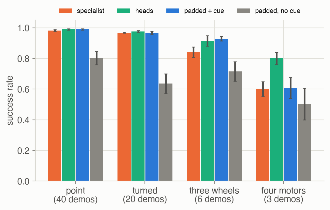
Trained alone, the robots with plenty of data do well, and the one with 3 episodes reaches the goal in 60% of held-out tasks (Figure 2). Trained together, with a separate output head per robot, four motors rises to 80% and three wheels from 84% to 91%, while the two data-rich robots lose nothing. The shared layers learn how to get round the post from everyone’s demos; each head only has to learn its robot’s motor mapping, which is far less to learn from 3 episodes. That is positive transfer. It is not guaranteed: four motors gained in 7 of the 8 seeds, not all of them.
What to watch for. The table and the tasks stay the same throughout; only the network driving four motors changes. Trained on its own 3 demos, the specialist steers many runs from the upper starts into the post’s upper-left side: 8 of the 20 runs end at the post, and 11 reach their goals. After pooling, the network has learned how to get round the post from all four robots’ demos, and its four-motors head only converts that into this robot’s four motor commands: 15 runs reach their goals and 5 touch the post. Seed 0 is the seed whose gain from pooling is closest to the average over 8 seeds; the bar chart above shows the averages.
Robotics as sequence modeling
A VLM maps an image and a question to text: “what is in this picture?” → “the Statue of Liberty”. A robot policy maps an image and an instruction to actions. Squint, and the second is the first with a different kind of answer ▶ 13:02. So the generalist designs treat robotics as multimodal sequence modeling: turn everything into tokens and train a transformer ▶ 13:34. Gato, from Week 8’s guest, did this most literally: Atari frames, text, joint torques and button presses all became integers in one vocabulary.
Octo was the first open-source generalist policy, trained on 800,000 OXE trajectories ▶ 14:05. A language model encodes the instruction into task tokens; a shallow CNN turns image patches into observation tokens; a transformer much like a ViT processes them ▶ 15:08. Attention is block-wise causal: observation tokens see the task and earlier time steps, never later ones ▶ 16:10. Extra readout tokens collect what the actions need, and a diffusion head turns them into an action chunk ▶ 16:41 ▶ 17:44. It is trained by goal-conditioned behavior cloning, so the goal can be an image or an instruction.
Two practical choices mattered. Octo did not align coordinate frames across data sets, which kept it scalable, but it did align the gripper command: early failures were mostly grasps at the wrong moment, because data sets encoded “open” and “closed” four different ways ▶ 18:45. And it was meant to be fine-tuned: a new sensor, such as a force-torque reading, enters as a few new tokens, a new action space gets a new head, and since most parameters sit in the transformer, most of the knowledge survives ▶ 22:58. Fine-tuning a generalist worked much better than starting from the best pretrained visual representations ▶ 24:01.
One network, many bodies
How does one network output actions for robots with 7, 14 or 2 action dimensions, at 5 or 50 Hz? There are two designs ▶ 45:49. CrossFormer gives each kind of embodiment its own action head on a shared transformer, so each head can predict a chunk of its own length and rate ▶ 28:11; one checkpoint drove arms, bimanual robots, quadrupeds, wheeled robots and drones, and matched the specialists ▶ 30:15. π0 has a single action expert writing into one padded action space as large as the biggest robot’s; smaller robots pad with zeros ▶ 46:51.
Then how does the network know which robot it is driving? With heads, it does not need to: the user picks the head ▶ 50:01. With one padded output, the model has to infer the robot from what it sees: the camera views, the joint readings it gets as input, even the instruction (“cut the sushi” is not a task for a vacuum robot) ▶ 50:33. The toy’s padded network gets a one-hot cue standing in for those signals. With the cue it matches the heads on three of the robots; without it, it fails on every robot (Figure 2), because positions and goals alone do not say whose motors are attached. On four motors it did no better than the specialist (61%), possibly because its fourth output is trained by four motors’ 3 episodes alone, while the heads network gives each robot its own output weights on shared features; we have not tested this further.
Pretraining pays most when data are scarce
Does pretraining on many tasks actually help a new one? Many believed so, but it was hard to show in robotics ▶ 30:46. TRI’s large-behavior-model study tested it with blind, randomized real-robot trials and found pretraining made fine-tuning about 3 to 5 times more sample efficient, with the largest gains when the new task had little data ▶ 32:50. It also found that how the data were normalized often mattered more than architecture or algorithm ▶ 33:20. (The 3 to 5 times is the lecturer’s summary; we checked only the paper’s abstract, which says new tasks are learned with less data but gives no single factor.)
The toy reproduces the pattern. A fifth robot arrives with a handful of demos. Either train a network on them from scratch, or keep the pooled network frozen and fit only a new linear head on its features.
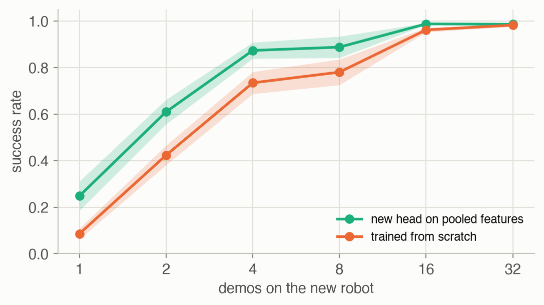
With 1 demo, the pooled features give 25% against 9%; with 4, 87% against 73% (Figure 5). Interpolating, the pooled network reaches 85% success with about 3.8 demos and the scratch network needs about 10.4, 2.8 times as many. By 32 demos the two are equal: with enough data of its own, the new robot no longer needs the others.
Start from a vision-language model
Even a million robot episodes are tiny next to what vision-language models are trained on, so the next question was whether internet-scale knowledge transfers to control ▶ 33:51. LLaVA showed the template: put image tokens in front of the text and let the language model attend over both ▶ 34:22. Treat actions the same way: turn them into tokens, add them to the vocabulary (overwriting the least used tokens), and fine-tune with the usual next-token loss ▶ 35:24. RT-2 and OpenVLA did this with the simple per-dimension binning of Week 7 ▶ 36:26.
The recipe many labs now follow comes from π0.5 and knowledge insulation ▶ 51:35. The VLM backbone is trained by next-token prediction on FAST-tokenized robot actions and web data; the web data keep it from forgetting what it knew ▶ 52:37. A separate action expert produces continuous actions by flow matching (Week 6); it reads the backbone, but a stop-gradient keeps its gradients out of it, which protects the VLM’s knowledge and speeds up training ▶ 53:08.
Feeding the model: batches and buffers
Pooled data break the simple assumption that every sample has the same shape. One data set has a single third-person camera, another adds two wrist cameras ▶ 39:03. Padding every sample to the longest one is easy, but in a mixed batch much of the compute goes on zeros ▶ 40:05. Sequence packing lays the samples end to end instead, so every token is real; the price is bookkeeping: the start of each sample, an attention mask that keeps samples from looking at each other, and positions that restart at each sample ▶ 40:35 ▶ 41:39. In the page’s example batch, two samples with 1 camera and two with 3, padding computes 232 tokens for 168 real ones, 28% wasted (worked example).
How randomly the loader mixes data mattered as much. Octo streamed trajectories from disk into a shuffle buffer and drew batches from it; with a buffer of 20,000 frames, batches held frames from too few trajectories and the policy generalized poorly, and enlarging it to 500,000 made a large difference with nothing else changed ▶ 42:41 ▶ 43:43. The toy streams 5,000 trajectories of 100 frames and draws batches of 256.
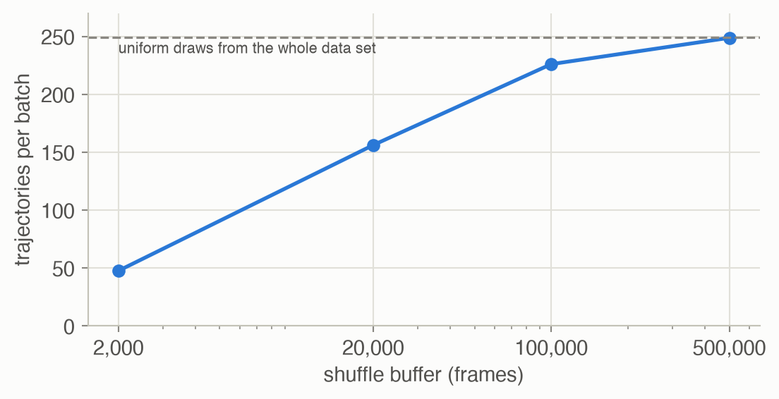
A batch from a 2,000-frame buffer holds frames from only 48 trajectories on average, so each gradient step sees a few situations many times over; a 20,000-frame buffer gives 156, and only a buffer near the size of the data set approaches the 250 of truly random draws (Figure 7). Loading by random reads from a flat index avoids the problem at the price of fast storage ▶ 44:14.
Learning from data of mixed quality
Pooling also mixes skill levels: careful demos, hesitant ones, the robot’s own failed attempts. Cloning all of it copies the average, mistakes included. This week’s guest showed that adding the lowest-quality data hurt π0.7 when the model was not told about quality, and helped when each episode came with metadata on its speed and quality ▶ 10:33. The discussion paper π*0.6 does this per action: a value function estimates each action’s advantage, the policy is trained on all data with one more input saying whether the advantage beat a threshold, and at test time it is asked for the good actions. Unlike filtering, nothing is thrown away: the bad steps still teach what the situations look like. The corridor example works this out exactly.
Evaluate in simulation, for rankings
A generalist must be tested on many tasks and robots, and real evaluation is slow and fragile: someone bumps a camera, a motor is replaced and the joint readings shift, and a single trial takes minutes ▶ 54:10 ▶ 55:13. Simulation is cheaper and reproducible ▶ 56:47. SIMPLER evaluates policies trained only on real data in simulated copies of the real setups ▶ 57:18, after narrowing two gaps: the control gap, by system identification so that the simulated arm responds to commands like the real one ▶ 58:52, and the visual gap, by green-screening real backgrounds behind simulated objects and projecting real textures onto them ▶ 59:23. What it promises is a ranking, not absolute numbers: 50% in simulation does not mean 50% on the robot, but if policy A beats B in SIMPLER, it should on the real robot too ▶ 60:55.
The second toy tests the control gap only. Nine policies, from 3 cloning budgets each run at 3 speed factors, are scored on the “real” point robot, whose motors are noisy, and in simulators whose motor gain is wrong (0.4 instead of 1) or estimated by system identification from 100 test commands.
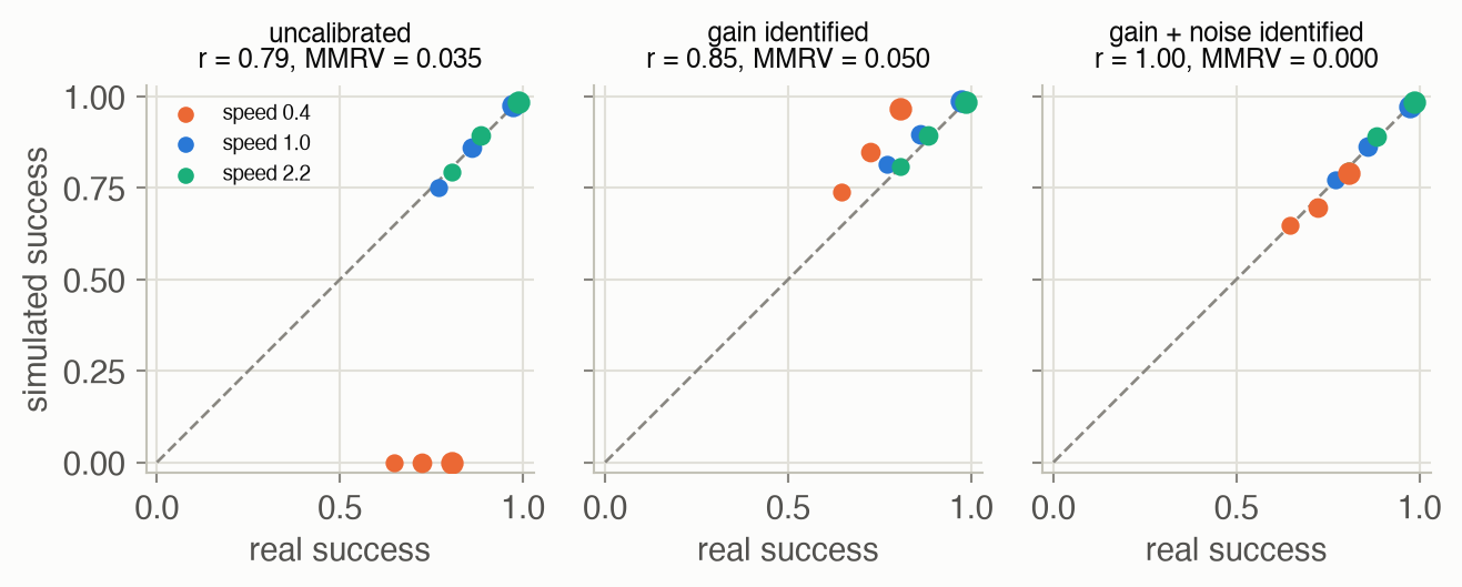
The uncalibrated simulator is badly wrong in absolute terms, 0.24 too low on average, because its weak motors leave the slowest policies far short of their goals: they score 0 in simulation and between 65% and 81% on the real robot (Figure 8). Identifying the gain brings the average much closer (now 0.05 too high) but not the ranking, because the simulator still lacks the motor noise, which hurts slow policies most: they now look 0.09 to 0.16 better in simulation than on the robot. With gain and noise identified, simulated and real success agree for every policy. Over 5 policy families the pattern holds: correlation 0.64–0.87 uncalibrated, 0.46–0.92 with the gain alone, and at least 0.967 fully calibrated. In this toy calibration closes the gap completely because the simulator’s model has the same form as the “real” robot; real setups always keep some gap, which is why SIMPLER reports rankings.
Key concepts & formulae
The lecture writes \(o_t\) for observations, \(a_t\) for actions and \(\ell\) for a language instruction; \(g\) is a goal, an image or an instruction. The ADM book writes the cloning objective as maximum likelihood over expert state-action pairs, the same thing without the goal.
Training on many robots
\[ \mathcal{L}(\theta) = -\,\mathbb{E}_{(o_{t-h:t},\, g,\, a_{t:t+H-1}) \sim \mathcal{D}} \big[\log \pi_\theta(a_{t:t+H-1} \mid o_{t-h:t}, g)\big] \tag{1}\]
In words. Make the demonstrated chunk of actions likely, given a short history of observations and the goal.
Term by term.
- \(o_{t-h:t}\): the last \(h+1\) observations (Octo uses a short window).
- \(g\): a goal image, or an instruction \(\ell\); one model learns to accept either.
- \(a_{t:t+H-1}\): a chunk of \(H\) actions (Week 7); Octo’s diffusion head models its distribution, so the log-likelihood is replaced by the denoising loss of Week 6.
- \(\mathcal{D}\): the pooled data of all robots and tasks.
\[ \mathcal{L}(\theta, f_1, \dots, f_K) = \frac{1}{K}\sum_{k=1}^{K} \mathbb{E}_{(\tau, c) \sim \mathcal{D}_k} \Big[ \textstyle\sum_{t} -\log \pi_\theta\big(a_t \mid s_t, f_k(c)\big) \Big] \tag{2}\]
In words. Several data sets describe tasks in different ways; each gets its own encoder into one shared goal space, and one policy learns from all of them.
Term by term.
- \(\mathcal{D}_k\): data set \(k\), demonstrations \(\tau\) paired with a task description \(c\) of kind \(k\): a goal image from hindsight relabelling, or a sentence.
- \(f_k\): the encoder for kind \(k\); all map into the same latent goal \(z = f_k(c)\).
- Why it pays: goal images come free (the last frame of any window), sentences cost an annotator; in Lynch and Sermanet’s paper under 1% of the data needed language.
\[ \mathcal{L}(\theta) = \frac{1}{N} \sum_{i=1}^{N} \sum_{j=1}^{D} m_{ij}\,\big(\hat a_{ij} - a_{ij}\big)^2, \qquad m_{ij} \in \{0, 1\} \tag{3}\]
In words. The network outputs \(D\) numbers per sample; only the entries that belong to this sample’s robot count.
Term by term.
- Padded action space (π0): \(D = \max_e d_e\); robot \(e\) fills the first \(d_e\) entries and \(m_{ij} = 0\) for the rest.
- Separate heads (CrossFormer): \(D = \sum_e d_e\), each robot owns a block of columns, and \(m_{ij} = 1\) only on that block. Since the last layer is linear, a block of its columns is a separate head reading shared features.
- Numeric check: the toy’s heads network has 11 outputs (2 + 2 + 3 + 4); a four-motors sample trains only the last four and leaves the other heads’ weights untouched.
Tokens for everything
\[ \mathcal{L}(\theta) = -\sum_{b=1}^{B} \sum_{l=1}^{L} m(b, l)\, \log p_\theta\big(s^{(b)}_l \mid s^{(b)}_1, \dots, s^{(b)}_{l-1}\big) \tag{4}\]
In words. Next-token prediction over a flat token sequence of text, image patches, observations and actions, scoring only text and action tokens.
Term by term.
- \(s^{(b)}_l\): token \(l\) of training sequence \(b\), from one shared vocabulary.
- \(m(b, l)\): 1 if the token is text or an action, 0 for image and observation tokens, which are context only.
- Tasks are told apart by prompting with a demonstration of the same task, not by a task id.
\[ F(x) = \operatorname{sgn}(x)\,\frac{\log(|x|\,\mu + 1)}{\log(M\mu + 1)}, \qquad \mu = 100,\; M = 256 \tag{5}\]
In words. Squeeze a real number into \([-1, 1]\) on a roughly logarithmic scale, so small values keep fine resolution and large ones share coarse bins.
Term by term.
- Borrowed from audio coding (and WaveNet); Gato applies it to continuous observations, clips to \([-1, 1]\), cuts that range into 1,024 equal bins, and shifts the bin index past the 32,000 text tokens.
- Numeric check: \(F(0.01) =\) 0.0683, so 1% of the input scale takes about 7% of the output range (worked example).
Batching heterogeneous samples
\[ \text{waste} = 1 - \frac{\sum_{i=1}^{B} L_i}{B \cdot \max_i L_i} \tag{6}\]
In words. The share of computed tokens that are padding, when every sample is padded to the longest.
Term by term. \(L_i\): tokens in sample \(i\); \(B\): samples in the batch. Attention costs grow with the square of the padded length, so the wasted share of attention compute is larger still.
\[ \begin{aligned} c_i &= \textstyle\sum_{j < i} L_j \quad (\texttt{cu\_seqlens}) \\ M_{pq} &= \mathbb{1}[\,\mathrm{seg}(p) = \mathrm{seg}(q)\,] \\ \mathrm{pos}(p) &= p - c_{\mathrm{seg}(p)} \end{aligned} \tag{7}\]
In words. Lay the samples end to end; remember where each starts; let a token attend only within its own sample; and number positions from 0 again in every sample.
Term by term.
- \(\mathrm{seg}(p)\): which sample token \(p\) belongs to; \(M\) is block-diagonal (a causal model also needs \(q \le p\)).
- Without the mask, a sample attends to its neighbours’ images; without the position reset, the fourth sample’s first token sits at a position no unpacked sample ever has.
- Numeric check: in the toy batch, packed attention with the mask matches per-sample attention to 3e-16; without it the outputs differ by up to 0.73.
From VLM to VLA
\[ \mathcal{L} = \underbrace{\mathcal{L}_{\text{next token}}\big(\text{language, FAST tokens; robot + web data}\big)}_{\text{trains the VLM backbone}} \;+\; \lambda\, \underbrace{\mathcal{L}_{\text{flow}}\big(v_\phi(\cdot \mid \mathrm{sg}[h_\theta])\big)}_{\text{trains the action expert only}} \tag{8}\]
In words. The backbone learns from discrete tokens, robot and web alike; the continuous action expert learns flow matching while reading the backbone’s features as constants.
Term by term.
- \(h_\theta\): the backbone’s internal features; \(\mathrm{sg}[\cdot]\): stop-gradient, so \(\mathcal{L}_{\text{flow}}\) changes \(\phi\) but not \(\theta\).
- \(v_\phi\): the action expert’s velocity field (Week 6’s flow matching).
- FAST tokens (Week 7) give the backbone a robot-action target it can learn by next-token prediction.
- \(\lambda\): a weight between the two losses. The equation is a schematic of the lecture’s summary; the paper gives the exact objective.
- Why: the knowledge-insulation paper finds that letting the action expert’s gradients into the VLM slows training and loses the VLM’s semantic knowledge.
Training tips from the lecture. For a VLA with action tokens, wait until teacher-forced action-token accuracy reaches about 95% before trying the robot; below that, rollouts will not be good ▶ 37:29. Teacher-forced accuracy is not rollout performance, so also track the L1 and L2 error of the decoded continuous actions ▶ 38:32.
Learning from experience
\[ \begin{aligned} A(o_t, a_t) &= \textstyle\sum_{t'=t}^{t+N-1} r_{t'} + V(o_{t+N}) - V(o_t), \qquad I_t = \mathbb{1}\big[A(o_t, a_t, \ell) > \epsilon_\ell\big] \\ \min_\theta\; &\mathbb{E}_{\mathcal{D}}\big[-\log \pi_\theta(a_t \mid o_t, \ell) - \alpha \log \pi_\theta(a_t \mid I_t, o_t, \ell)\big] \end{aligned} \tag{9}\]
In words. Score each recorded action by how much better than usual it did, label it good or not, train one policy on all actions with that label as an extra input, and ask for “good” at test time.
Term by term.
- \(V\): a value function of the data’s own behavior, fitted to observed returns (π*0.6 predicts steps to success).
- \(A\): an \(N\)-step advantage estimate, as in Week 5; \(\epsilon_\ell\): a per-task threshold.
- First term: plain cloning, which keeps the model able to represent all behavior; second term: cloning conditioned on the label, weighted by \(\alpha\).
- Human corrections during deployment are always labelled good.
- Why it holds: the paper shows that conditioning on “improvement” yields a policy that does at least as well as the data’s behavior, for a monotone notion of improvement; in the special case of their \(\beta = 1\), the improved policy is exactly \(\pi(a \mid I = 1, o, \ell)\).
Evaluating
\[ \mathrm{MMRV} = \frac{1}{N}\sum_{i=1}^{N} \max_{j}\; |R_i - R_j| \cdot \mathbb{1}\big[(R_{S,i} < R_{S,j}) \neq (R_i < R_j)\big] \tag{10}\]
In words. For each policy, find the worst pair the simulator orders the wrong way round, measured by how far apart the two really are; average over policies.
Term by term.
- \(R_i\), \(R_{S,i}\): real and simulated success of policy \(i\). MMRV = 0 means no pair is misordered.
- A swap of two policies that are really 0.01 apart costs little; a swap of policies 0.3 apart costs a lot. Pearson’s \(r\) instead rewards a linear relation, and can penalize a simulator that ranks correctly but nonlinearly.
- Numeric check: the toy’s uncalibrated simulator has MMRV 0.035 and \(r\) = 0.79; identifying the gain alone raises \(r\) to 0.85 but worsens MMRV to 0.050: the two metrics can disagree.
\[ \hat k = \frac{\sum_i a_i \cdot \Delta x_i}{\Delta t \sum_i a_i \cdot a_i}, \qquad \hat\sigma = \operatorname{std}\Big(\frac{\Delta x_i}{\Delta t} - \hat k\, a_i\Big) \tag{11}\]
In words. Send known commands to the real robot, measure how far it moves, and fit the simulator’s gain by least squares; what the fit cannot explain is the noise.
Term by term. \(a_i\): a test command; \(\Delta x_i\): the measured motion over one step \(\Delta t\). SIMPLER fits arm controller parameters the same way, matching simulated to real end-effector trajectories. Numeric check: from 100 commands the toy finds \(\hat k\) = 0.957 and \(\hat\sigma\) = 0.306 (true: 1 and 0.3).
\[ \mathrm{SE}(\hat p) = \sqrt{\frac{\hat p\,(1 - \hat p)}{n}} \tag{12}\]
In words. A success rate measured from \(n\) independent trials is uncertain by about this much.
Term by term. With \(\hat p = 0.5\) and \(n = 20\) trials, SE \(= 0.11\): two policies 10 points apart cannot be told apart. This is why real-robot comparisons need many trials, blind scoring and randomized order, as in TRI’s study, and why cheap simulated trials are attractive.
Worked examples
Example 1: padding against packing
Two samples from a data set with one camera and two from a data set with three; each image gives 16 tokens and language plus actions add 10.
| sample | cameras | tokens \(L_i\) | starts at \(c_i\) | positions |
|---|---|---|---|---|
| 1 | 1 | 26 | 0 | 0 … 25 |
| 2 | 1 | 26 | 26 | 0 … 25 |
| 3 | 3 | 58 | 52 | 0 … 57 |
| 4 | 3 | 58 | 110 | 0 … 57 |
Padded, the batch is \(4 \times\) 58 \(=\) 232 tokens, of which 168 are real: Equation 6 gives 28% waste. Packed, it is one sequence of 168 tokens with cu_seqlens = [0, 26, 52, 110, 168]. Token 52 is the first of sample 3, so its position is reset to 0, not 52, and the block-diagonal mask lets it attend to tokens 52–109 only. Attention on this packed sequence then equals attention on each sample alone (difference 3e-16); drop the mask and it differs by up to 0.73.
Example 2: Gato’s tokens for continuous values
| value \(x\) | \(F(x)\) | bin (of 1,024) | token id |
|---|---|---|---|
| -2 | -0.5225 | 244 | 32,244 |
| -0.05 | -0.1765 | 421 | 32,421 |
| 0 | +0.0000 | 512 | 32,512 |
| 0.01 | +0.0683 | 546 | 32,546 |
| 0.05 | +0.1765 | 602 | 32,602 |
| 0.5 | +0.3874 | 710 | 32,710 |
| 3 | +0.5623 | 799 | 32,799 |
The values 0.01 and 0.05 are only 0.04 apart but land 56 bins apart; 0.5 and 3.0 are 2.5 apart and land 89 bins apart. Mu-law spends resolution where values are small, which suits joint velocities and torques that are usually small but occasionally large. Every token id is at least 32,000, so the model can never confuse a joint reading with a word.
Example 3: advantage conditioning in a corridor
A corridor of 10 cells, the goal at the end. Operators step forward with probability 0.8 and back with probability 0.2 (at cell 0 they stay put); every step costs \(-1\). Solving the value equations exactly:
| cell \(s\) | \(V(s)\) | \(A(s, \text{forward})\) | \(A(s, \text{back})\) |
|---|---|---|---|
| 0 | -16.11 | +0.25 | -1.00 |
| 1 | -14.86 | +0.56 | -2.25 |
| 2 | -13.30 | +0.64 | -2.56 |
| 5 | -8.33 | +0.67 | -2.67 |
| 8 | -3.33 | +0.67 | -2.67 |
| 9 | -1.67 | +0.67 | -2.67 |
Every forward step has a positive advantage and every back step at most \(-1\), so the label \(I = \mathbb{1}[A > 0]\) separates them exactly. Plain cloning learns the operators’ own mix and needs 16.1 steps on average to reach the goal; the policy conditioned on \(I = 1\) steps forward every time and needs 10. Filtering whole episodes would keep only those with no back step at all: a fraction \(0.8^{10}\) = 10.7% of them. Advantage conditioning keeps every step, and in a real task the “bad” steps still show the policy what the world looks like from where mistakes lead. (A first version of this page’s toy tried to learn the value function from noisy 2D demos; its one-step labels were only about 80% right, not enough to beat filtering, which is why this example uses the exact values. π*0.6 trains a large value function on far more data.)
Interactive
A new robot, one demo at a time
What to try. Start at 1 demo: one demonstration is too little for either network (1 and 4 of 20 succeed), since even the pooled network must learn the new robot’s whole motor mapping from 60 time steps. Step to 4: the pooled network, which only has to fit that mapping, succeeds on 16 of 20 against 13 for the network that must also learn how to get round the post. From 16 demos on both succeed on all 20: plenty of the robot’s own data makes the pooled knowledge unnecessary.
Calibrating a simulator
The nine policies of Figure 8, scored in a simulator whose motor gain you choose. The real robot’s gain is 1 and its motor noise has standard deviation 0.3; system identification estimated 0.96 and 0.31.
What to try. Start at gain 0.4 with no noise: the slow policies (orange) score 0 in simulation, and \(r\) is 0.79. Raise the gain to 1, the real value: the slow policies come back, but without noise every dot sits on or above the diagonal, the slow ones most (\(r\) = 0.82, mean 0.89 against 0.83 real). Now switch the noise on: the dots fall onto the diagonal (\(r\) = 1.00). Push the gain past 1.2 and watch which policies the simulator starts to flatter.
Algorithm & code
One network, many robots
def fit_masked(params, X, Y, M, steps, rng, alpha=0.003, batch=256):
    """Adam on the squared error over the entries where the mask M is 1.

    X (n, d_in), Y and M (n, d_out). Entries with M = 0 are padding or
    another robot's head: they get no gradient, so whatever the network
    outputs there is never trained. Every method gets the same number of
    gradient steps, whatever the size of its data."""
    opt = nn.Adam(params, alpha)
    for _ in range(steps):
        idx = rng.integers(0, len(X), min(batch, len(X)))
        Yh, cache = nn.forward(params, X[idx])
        m = M[idx]
        dY = 2 * m * (Yh - Y[idx]) / len(idx)       # zero where masked
        params = opt.step(params, nn.backward(params, cache, dY))
    return params

def train_heads(data, seed) -> list:
    """One network, one output head per robot (CrossFormer style).

    The last layer is linear, so a block of its output columns is a
    separate linear head reading the same hidden features. Each sample
    is masked to its own robot's block: only that head, and the shared
    layers below it, learn from it. data: name -> (obs, act)."""
    cols = head_slices()
    n_out = sum(J.shape[1] for J in ROBOTS.values())
    obs, Y, M = [], [], []
    for name, (o, a) in data.items():
        y, m = np.zeros((len(o), n_out)), np.zeros((len(o), n_out))
        y[:, cols[name]], m[:, cols[name]] = a, 1.0
        obs.append(o), Y.append(y), M.append(m)
    rng = np.random.default_rng(seed)
    params = nn.init_mlp([4, HIDDEN, HIDDEN, n_out], rng)
    return fit_masked(params, np.concatenate(obs), np.concatenate(Y),
                      np.concatenate(M), STEPS, rng)

def train_padded(data, seed, cue_on=True) -> list:
    """One network with one padded output of size D_MAX (pi0 style).

    A robot with d < D_MAX motors fills the first d outputs; the rest
    are padding, masked out of the loss. Nothing in the output says
    which robot is driven, so the network must infer it from its input:
    position, goal and, if cue_on, the embodiment cue."""
    obs, Y, M = [], [], []
    for name, (o, a) in data.items():
        y, m = np.zeros((len(o), D_MAX)), np.zeros((len(o), D_MAX))
        y[:, :a.shape[1]], m[:, :a.shape[1]] = a, 1.0
        obs.append(np.c_[o, cue(name, len(o), cue_on)])
        Y.append(y), M.append(m)
    rng = np.random.default_rng(seed)
    params = nn.init_mlp([4 + len(ROBOTS), HIDDEN, HIDDEN, D_MAX], rng)
    return fit_masked(params, np.concatenate(obs), np.concatenate(Y),
                      np.concatenate(M), STEPS, rng)

def fit_new_head(params, obs, act, ridge=1e-3) -> tuple[Array, Array]:
    """A new linear head on frozen pooled features, by ridge regression:
    solves (H'H + ridge I) w = H'a, with a column of ones for the bias.
    Returns (W (H, d), b (d,))."""
    H = np.c_[features(params, obs), np.ones(len(obs))]
    w = np.linalg.solve(H.T @ H + ridge * np.eye(H.shape[1]), H.T @ act)
    return w[:-1], w[-1]
import numpy as np
import torch
import torch.nn as nn
from rlc.toys import w09_generalist as w9
torch.manual_seed(0)
class MultiHeadPolicy(nn.Module):
"""Shared trunk, one linear head per robot (CrossFormer style)."""
def __init__(self, action_dims: dict, hidden=64):
super().__init__()
self.trunk = nn.Sequential(nn.Linear(4, hidden), nn.Tanh(),
nn.Linear(hidden, hidden), nn.Tanh())
self.heads = nn.ModuleDict({name: nn.Linear(hidden, d)
for name, d in action_dims.items()})
def forward(self, obs, robot):
return self.heads[robot](self.trunk(obs)) # (B, d_robot)
names = {k: k.replace(" ", "_") for k in w9.ROBOTS} # ModuleDict keys
data = {names[k]: tuple(torch.tensor(x, dtype=torch.float32) for x in v)
for k, v in w9.pooled_data(0).items()} # obs (n, 4), act (n, d)
policy = MultiHeadPolicy({k: a.shape[1] for k, (_, a) in data.items()})
opt = torch.optim.Adam(policy.parameters(), lr=3e-3)
# Each step takes a batch from every robot, so the trunk sees all of
# them; each loss term reaches only its own head (the masking of the
# NumPy version, done by indexing instead).
losses = []
for step in range(1500):
loss = 0.0
for robot, (obs, act) in data.items():
idx = torch.randint(len(obs), (64,))
loss = loss + ((policy(obs[idx], robot) - act[idx]) ** 2).sum(1).mean()
opt.zero_grad(); loss.backward(); opt.step()
losses.append(loss.item())
assert np.mean(losses[-50:]) < 0.2 * np.mean(losses[:50])
# A new robot: freeze the trunk, fit only a fresh head on 4 demos.
obs, act = (torch.tensor(x, dtype=torch.float32) for x in
w9.demos(w9.NEW_ROBOT, 4, np.random.default_rng(1)))
policy.trunk.requires_grad_(False)
policy.heads["new"] = nn.Linear(64, act.shape[1])
opt = torch.optim.Adam(policy.heads["new"].parameters(), lr=1e-2)
for step in range(500):
loss = ((policy(obs, "new") - act) ** 2).sum(1).mean()
opt.zero_grad(); loss.backward(); opt.step()
assert loss.item() < 0.05, loss.item()In the NumPy version, one output layer holds every robot’s columns and a mask picks the right block; the PyTorch version gives each robot its own nn.Linear and indexes by name. The two are the same model. requires_grad_(False) freezes the trunk in place (the trailing underscore marks an in-place method), so the new head trains on fixed features, as fit_new_head does by ridge regression.
Packing a batch
def pack(lengths) -> tuple[Array, Array, Array]:
    """Sequence packing: samples laid end to end in one sequence.

    Returns cu_seqlens, the prefix sums [0, L1, L1 + L2, ...] that mark
    where each sample starts; seg, the sample index of every token; and
    pos, every token's position within its own sample (it restarts at 0
    at each boundary)."""
    lengths = np.asarray(lengths)
    cu = np.r_[0, np.cumsum(lengths)]
    seg = np.repeat(np.arange(len(lengths)), lengths)
    pos = np.arange(cu[-1]) - cu[seg]
    return cu, seg, pos

def attend(q, k, v, allowed) -> Array:
    """Softmax attention, q k v (n, d), allowed (n, n) boolean: query i
    may look at key j only where allowed[i, j]."""
    s = q @ k.T / np.sqrt(q.shape[1])
    s = np.where(allowed, s, -np.inf)
    w = np.exp(s - s.max(1, keepdims=True))
    return (w / w.sum(1, keepdims=True)) @ v

def packing_check(lengths, d=8, seed=0) -> dict:
    """Attention over a packed sequence, with and without the
    block-diagonal mask, against attention over each sample on its own.
    Returns the largest difference from the per-sample result for each."""
    rng = np.random.default_rng(seed)
    cu, seg, _ = pack(lengths)
    q, k, v = (rng.normal(size=(cu[-1], d)) for _ in range(3))
    alone = np.concatenate([attend(q[a:b], k[a:b], v[a:b],
                                   np.ones((b - a, b - a), bool))
                            for a, b in zip(cu[:-1], cu[1:])])
    block = seg[:, None] == seg[None, :]
    full = np.ones_like(block)
    return {"block-diagonal": float(np.abs(attend(q, k, v, block)
                                           - alone).max()),
            "no mask": float(np.abs(attend(q, k, v, full) - alone).max())}
import torch.nn.functional as F
torch.manual_seed(0)
lengths = torch.tensor([26, 26, 58, 58]) # tokens per sample
cu_seqlens = torch.cat([torch.zeros(1, dtype=torch.long),
lengths.cumsum(0)]) # [0, 26, 52, 110, 168]
seg = torch.repeat_interleave(torch.arange(len(lengths)), lengths) # (T,)
pos = torch.arange(len(seg)) - cu_seqlens[seg] # restarts at 0 per sample
T, H, D = len(seg), 2, 16 # tokens, heads, head dim
q, k, v = torch.randn(3, 1, H, T, D).unbind(0) # each (1, H, T, D)
# Boolean mask, True = may attend: same sample only (block-diagonal).
# Broadcasts over batch and heads: (T, T) -> (1, H, T, T).
allowed = seg[:, None] == seg[None, :]
packed = F.scaled_dot_product_attention(q, k, v, attn_mask=allowed)
# Reference: attend within each sample separately, then concatenate.
alone = torch.cat([F.scaled_dot_product_attention(q[..., a:b, :], k[..., a:b, :],
v[..., a:b, :])
for a, b in zip(cu_seqlens[:-1], cu_seqlens[1:])], dim=2)
leaky = F.scaled_dot_product_attention(q, k, v) # no mask
assert torch.allclose(packed, alone, atol=1e-5)
assert (leaky - alone).abs().max() > 0.1
assert pos[cu_seqlens[2]] == 0 and pos.max() == lengths.max() - 1Kernels such as FlashAttention’s variable-length mode take cu_seqlens directly and never build the \(T \times T\) mask; the dense mask here is for clarity. Positions must come from pos, not from torch.arange(T): with rotary or learned positional encodings, a token’s position is part of its input.
Papers
Papers discussed in class
Key papers from the lecture
Guest spotlight
Quan Vuong (co-founder of Physical Intelligence; earlier at Google DeepMind, where he started and co-led the RT-X and Open X-Embodiment projects) presented π0.7, whose main claim is a single model that performs many tasks at specialist level ▶ 01:01. That matters for scaling: until now, top performance on a task meant post-training a model for that task, and every extra checkpoint is one more thing to manage ▶ 01:32. It is hard because more data does not automatically mean a better model: train on everything you have and you usually get something worse than a carefully tuned specialist ▶ 02:34. He showed a symptom: a policy imitating teleoperation data was slower than the teleoperators themselves, while online RL made it faster than them ▶ 03:37.
The architecture is close to π0.5 and π0.6: a language model and a pretrained vision encoder with an action expert grafted on, prompted with the task, optionally a subtask, and metadata on the speed and quality of each training episode, plus a new ability to condition on goals ▶ 05:10. A separate high-level component, a person or a planner, proposes subtasks but never actions ▶ 06:45. One checkpoint matched or beat RL- and SFT-tuned specialists on laundry, tiny screws, box assembly and taking out the trash ▶ 08:23. His explanation for beating them: in real-robot evaluation every test is partly a generalization test, since something in the scene always changes, and a generalist is more robust to such changes ▶ 09:25. The metadata result is this page’s quality story: adding the lowest-quality data lowered performance without metadata and raised it sharply with metadata ▶ 10:33. Shirt folding learned on one robot pair transferred to a bimanual UR5 station that had no folding data at all ▶ 12:39, and a person coaching in language led it through tasks it had no data for ▶ 14:10.
He also described deployment with partner companies, such as folding customers’ laundry in a laundromat and packing orders through a full working day, where the question is whether remote interventions become rare enough to break even ▶ 16:47 ▶ 19:53, and said the open-sourced π0 and π0.5 weights are the same checkpoints the company’s researchers use ▶ 15:14. In the Q&A: multi-fingered hands are not yet cheap, reliable and easy to teleoperate all at once, so two-finger grippers serve research at scale better ▶ 21:57; what to scale (many tasks or many demos per task, human video, robots) is an open experimental question ▶ 25:34; whether VLAs or video action models scale better is undecided, with models heading from single-digit to tens of billions of parameters ▶ 30:15 ▶ 31:47; and home robots wait on model capability, since a robot that works in every home would mean physical intelligence is solved ▶ 24:34.
How it connects to this week. π0.7 is the lecture’s recipe pushed to the point where the generalist beats the specialists; its metadata conditioning and π*0.6’s advantage conditioning are the same move, telling the model about data quality instead of discarding the bad data; and the cross-embodiment folding result is positive transfer at full scale.
Solved problems
1. Padding a batch. A batch has 6 samples with one camera and 2 with three cameras; each image is 256 tokens and language plus actions add 20. How much of a padded batch is padding? What is cu_seqlens if you pack them in that order?
TipSolution
One camera: 276 tokens; three: 788. Real tokens: \(6 \cdot 276 + 2 \cdot 788 = 1656 + 1576 = 3232\). Padded: \(8 \cdot 788 = 6304\). Waste (Equation 6): \(1 - 3232/6304 \approx 49\%\): half the batch is zeros, the lecture’s warning. cu_seqlens = [0, 276, 552, 828, 1104, 1380, 1656, 2444, 3232].
2. Which robot am I? Two robots have the same cameras, the same 2-D action space and the same tasks, but one’s motor axes are mirrored. Your model has one padded action output. What happens, and what are two fixes?
TipSolution
Nothing in the input tells the robots apart, so the same observation is paired with two different correct actions; least-squares training averages them, and the average of an action and its mirror image moves the robot along only one axis or not at all, wrong for both robots (the toy’s “no cue” bars, Figure 2). Fixes: give the model a cue, such as an embodiment token, a camera view that shows the robot, or joint readings that differ; or use separate heads and let the user pick one, as CrossFormer does. Aligning the action spaces by hand also works, at the cost Octo and CrossFormer chose to avoid.
3. Is the new policy better? Policy A succeeded in 12 of 20 trials, policy B in 15 of 20. Is B better? How many trials per policy would make a 15-point gap at about these rates two standard errors of the difference?
TipSolution
\(\hat p_A = 0.6\), \(\hat p_B = 0.75\). Standard errors (Equation 12): \(\sqrt{0.6 \cdot 0.4/20} = 0.110\) and \(\sqrt{0.75 \cdot 0.25/20} = 0.097\); the difference has SE \(\sqrt{0.110^2 + 0.097^2} = 0.146\), so a 0.15 gap is about one SE: no evidence either way. For the gap to be two SEs, \(\sqrt{(0.24 + 0.1875)/n} \le 0.075\), so \(n \ge 0.4275 / 0.075^2 \approx 76\) trials per policy. That is hours of robot time for one comparison.
4. MMRV by hand. Three policies have real success 0.2, 0.5 and 0.6, and simulated success 0.3, 0.7 and 0.65. Compute the MMRV and the ranking error it describes.
TipSolution
Real order: 1 < 2 < 3. Simulated order: 1 < 3 < 2, so only the pair (2, 3) is misordered, and it costs \(|0.5 - 0.6| = 0.1\). Each policy’s worst violation: policy 1, none (0); policy 2, 0.1; policy 3, 0.1. MMRV \(= (0 + 0.1 + 0.1)/3 \approx 0.067\) (Equation 10). The simulator confuses two policies that are only 10 points apart in reality; it never confuses either with policy 1.
5. Advantage conditioning, quickly. Operators in a 20-cell corridor step forward with probability 0.9 and back with 0.1. Far from the start, how many steps per cell does a cloned policy take? What fraction of episodes would filtering keep if it kept only flawless ones, and how many steps does the advantage-conditioned policy take?
TipSolution
Each step moves forward on average \(0.9 - 0.1 = 0.8\) cells, so cloning takes about \(1/0.8 = 1.25\) steps per cell, about 25 steps for 20 cells (slightly fewer, since at cell 0 a back step cannot go further back). A flawless episode needs 20 forward steps in a row: \(0.9^{20} \approx 12\%\) of episodes. Forward steps have positive advantage and back steps negative, so conditioning on \(I = 1\) gives a policy that always steps forward: 20 steps, trained on all the data (Equation 9, Example 3).
Recap
- Generalists are built from pooled data. OXE combined over a million episodes from 22 robots, and one model trained on it beat the per-data-set methods. Why it matters: robot data are scarce, so every lab’s data has to count.
- One network can drive many bodies. Tokenize everything, share a transformer, and either give each robot a head (CrossFormer) or one padded action space whose robot the model infers (π0). Why it matters: it is how one checkpoint controls arms, quadrupeds and drones; in the toy it lifted the data-poor robot from 60% to 80%.
- Pretraining helps most when the new task has little data. Why it matters: it is the case for robot foundation models, and it sets expectations: with plenty of task data, the advantage fades.
- VLAs inherit web knowledge if you protect it. Actions as tokens, co-training with web data, and a stop-gradient between the VLM and the action expert. Why it matters: it is the recipe behind today’s strongest generalist policies and the guest’s π0.7.
- Data quality must be represented, not ignored. Metadata (π0.7) and advantage labels (π*0.6) let bad data help instead of hurt. Why it matters: deployment produces exactly such mixed data, and it is how these policies keep improving after launch.
- Evaluate by rankings. Real evaluation is slow and noisy; a calibrated simulator can rank policies reliably even when its absolute numbers are off. Why it matters: without cheap, trustworthy evaluation, no design choice in this list can be tested.
Cheat sheet & connections
| Name | Formula | Where |
|---|---|---|
| Goal-conditioned BC | \(-\log \pi(a_{t:t+H-1} \mid o_{t-h:t}, g)\) | Equation 1 |
| Multicontext imitation | one policy, encoder \(f_k\) per kind of task description | Equation 2 |
| Masked multi-robot loss | \(\sum_j m_{ij} (\hat a_{ij} - a_{ij})^2\) | Equation 3 |
| Gato’s loss | next-token loss on text and action tokens only | Equation 4 |
| Mu-law ★ | \(\operatorname{sgn}(x) \log(1 + \mu|x|) / \log(1 + M\mu)\) | Equation 5 |
| Padding waste | \(1 - \sum L_i / (B \max L_i)\) | Equation 6 |
| Packing | cu_seqlens, block-diagonal mask, positions reset | Equation 7 |
| VLA recipe | next-token loss + flow loss through \(\mathrm{sg}[h_\theta]\) | Equation 8 |
| Advantage conditioning | \(I_t = \mathbb{1}[A > \epsilon_\ell]\); clone with and without \(I\) | Equation 9 |
| MMRV | mean worst misordered real gap | Equation 10 |
| SysID | least-squares gain, residual noise | Equation 11 |
| Success-rate SE | \(\sqrt{\hat p (1 - \hat p) / n}\) | Equation 12 |
Common pitfalls.
- Pooling data without aligning what must be aligned: Octo had to unify gripper conventions, while TRI found normalization mattered more than architecture.
- Padding a batch where half the samples have three times the cameras, and paying for the zeros.
- Packing without a block-diagonal mask, or without resetting positions.
- A small shuffle buffer: batches full of frames from the same few trajectories.
- A padded action space with nothing in the input that identifies the robot.
- Fine-tuning a VLA’s action expert with gradients flowing into the VLM, and losing its knowledge.
- Cloning mixed-quality data as if it were all good, or filtering away most of it.
- Reading a simulator’s absolute success rates as predictions of real ones.
- Declaring one policy better from 20 trials each.
Connections. Week 3’s behavior cloning is the training objective here, now goal-conditioned and multi-robot. Week 5’s advantages return in π*0.6, used to label data rather than weight gradients. Week 6’s diffusion and flow matching are Octo’s head and π0’s action expert. Week 7’s tokenization, transformers and action chunks are the building blocks of every model on this page. Week 8’s guest led Gato, and the choice between VLM and video backbones is still open, as this week’s guest said. Week 10 asks how such policies can reason before acting. In the ADM Companion: behavioral cloning and advantage estimation.
Resources
- Lecture: video (1:03:28)
- Slides: Official slides (ETH; password-protected) · Community rebuild (unofficial, student repo)
- Guest lecture: Quan Vuong (Physical Intelligence), π0.7, A Generalist Model with Emergent Capabilities: video (36:59)
- Papers:
- Language Conditioned Imitation Learning over Unstructured Data (Lynch & Sermanet, 2021)
- A Generalist Agent (Reed et al., 2022)
- π*0.6: a VLA That Learns From Experience (Physical Intelligence, 2025)
- Open X-Embodiment: Robotic Learning Datasets and RT-X Models (Open X-Embodiment Collaboration, 2024)
- Octo: An Open-Source Generalist Robot Policy (Octo Model Team (Ghosh, Walke, Pertsch, Black, Mees et al.), 2024)
- Scaling Cross-Embodied Learning: One Policy for Manipulation, Navigation, Locomotion and Aviation (Doshi, Walke, Mees, Dasari & Levine, 2024)
- A Careful Examination of Large Behavior Models for Multitask Dexterous Manipulation (TRI LBM Team, 2025)
- π0: A Vision-Language-Action Flow Model for General Robot Control (Black et al. (Physical Intelligence), 2025)
- π0.5: a Vision-Language-Action Model with Open-World Generalization (Physical Intelligence (Black et al.), 2025)
- Knowledge Insulating Vision-Language-Action Models: Train Fast, Run Fast, Generalize Better (Driess et al., 2025)
- Evaluating Real-World Robot Manipulation Policies in Simulation (Li, Hsu, Gu, Pertsch, Mees et al., 2024)