Week 8 · World Models
Lecture of 13 April 2026 · guest: Scott Reed
Big picture
Where this week fits
Week 7 built policies that map what the robot sees, and what it was told, to actions. A policy answers “given where I am and what I want, what should I do?” This week’s models answer a different question: “given where I am and what I do, what happens next?” ▶ 14:46 That is a world model, a learned simulator. With one, a robot can try many plans in its head and carry out only the best, can train a policy in imagination instead of on hardware, and, if the model is built on video, can borrow knowledge of how the physical world moves from internet-scale data.
The question this week answers: how do you learn a model of what your actions will do, and how do you use it, for planning, for training policies, or as the backbone of the policy itself?
The key ideas at a glance
- A world model predicts consequences. It models the next state given the current state, an action and a memory of the past. A video model that is not conditioned on actions is, strictly, not a world model.
- Plan with it. Roll out candidate action sequences in the model, keep the best, execute the first step and replan from the next real observation (model predictive control). Pixel-space models showed this works but is costly and blurry.
- Errors compound, and planners exploit them. Each imagined step feeds on the last, so errors grow with the horizon; and an optimizer will find the actions where the model is most wrong in its favour.
- Imagine in a latent space. Compress observations into a small latent state, predict there, and train the policy entirely in imagination (Ha & Schmidhuber’s World Models, then PlaNet’s RSSM and the Dreamer line, up to Dreamer 4 obtaining diamonds in Minecraft from offline data).
- Scale to internet video. Video must be tokenized far more compactly than per-frame patches. Then the question is where actions live: as inputs (action-conditioned world models), as joint outputs with the video (world action models such as DreamZero), or decoded from video features by an inverse dynamics model (video action models such as mimic-video).
- Or skip the pixels. JEPA-style models predict the next embedding instead of the next frame, and must prevent the encoder from collapsing.
Vocabulary
| Term | Plain meaning |
|---|---|
| World model | A model of what happens next given the current state and an action, \(p(s_{t+1} \mid s_t, a_t, h_t)\) |
| Action-conditioned | Takes the action as an input, so you can ask “what if I do this?” |
| Model predictive control (MPC) | Plan a short sequence in the model, execute its first step, replan |
| Cross-entropy method (CEM) | Sample plans, keep the best, refit the sampling distribution, repeat |
| Imagination training | Improving a policy on rollouts of a learned model instead of the real world |
| Latent state | A compact vector summarizing an observation (and the past) |
| RSSM | Recurrent state-space model: a deterministic memory plus a stochastic latent, with a learned prior |
| Model exploitation | A planner or policy choosing actions where the model’s predictions are wrong in its favour |
| Video tokenizer | An encoder that turns video into far fewer tokens than per-frame patches |
| World action model (WAM) | One model that generates future video and actions together |
| Video action model (VAM) | A pre-trained video model whose features an inverse dynamics model decodes into actions |
| Inverse dynamics model (IDM) | Predicts the action that turned one observation into the next |
| JEPA | Joint-embedding predictive architecture: predict the next embedding, not the next image |
| Representation collapse | An encoder mapping every input to (nearly) the same vector, which makes prediction trivially easy |
After this week you can
- State what distinguishes a world model from a policy and from a plain video model.
- Plan with a learned model using CEM and replanning, and explain why replanning from real observations matters.
- Explain why prediction errors compound over a rollout and how a planner exploits model errors.
- Describe the World Models, RSSM and Dreamer designs and what each fixed.
- Estimate the token count of a video clip, and say how video tokenizers compress it.
- Compare action-conditioned world models, world action models and video action models.
- Explain representation collapse in JEPA-style models and three ways to prevent it.
Intuition
TipAnalogy
A batter facing a fastball has about 400 milliseconds before the ball reaches the plate, and the first 100 are spent just getting the image from eye to brain ▶ 12:50. There is no time to see where the ball is and then swing. Batters hit anyway because they predict where the ball will be and start swinging for that point ▶ 13:39. That internal prediction of what the world will do next is a world model, and it lets you act ahead of what your senses tell you.
A learned simulator
A policy maps a state and a goal to an action; a world model maps a state and an action to a distribution over next states ▶ 14:46. With one, the robot can imagine: roll out many candidate plans in the model, score them, and execute only the best, testing many hypothetical futures for the price of one real one ▶ 16:08. It plays the role of a physics simulator, but learned from data instead of built by hand ▶ 17:12. A hand-built simulator is fast and exact for what its authors modelled, such as rigid bodies, friction and collisions, and wrong for whatever they did not, such as cloth or tissue ▶ 17:54. A learned model captures whatever its data show, and nothing more.
The lecture’s definition is strict: a world model predicts the next state from the current state, an action and a memory of the past, and a video model that only takes text is not one ▶ 19:10. The action input is what makes it useful for control: it can answer “what if I do this?” ▶ 20:40
This page’s first toy is a puck on a table. Pushes move it, drag slows it, and a hill in the middle repels it; the puck cannot push straight over the hill and must go round. The agent does not know these dynamics. It has only transitions recorded while the puck was shoved around at random, and it fits a small neural network to them: that is its world model. With 4,000 transitions the one-step error is 0.0050, with 250 it is 0.0384 (averaged over 3 models each).
Planning in pixels
An early action-conditioned model worked directly on camera images. Predicting every pixel of the next frame is a hard generative problem, so Finn and colleagues predicted instead how each pixel would move under the planned action, and warped the current image accordingly ▶ 21:04. Visual Foresight used that model for model predictive control: the user marks a pixel and where it should go, the cross-entropy method samples and refines action sequences in the model, and the robot executes the first action and replans ▶ 22:17. The training data came from the robot’s own random interaction, with no labels ▶ 23:03. Its limits: a squared-error loss averages over uncertain futures and gives blurry predictions ▶ 24:04, errors accumulate as rollouts get longer, and evaluating whole image sequences for every candidate is expensive ▶ 24:26.
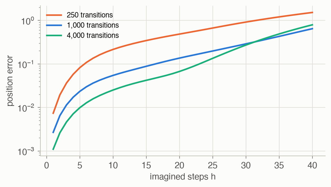
The puck toy shows the accumulation. Feed a model and the real table the same 40-step push sequence and compare where the puck ends up. With 1,000 transitions the average position error is 0.0027 after one step, 0.055 after 10 and 0.65 after 40 (Figure 2): every predicted step starts from the previous, slightly wrong, prediction. More data lowers the error over 20 steps, but not reliably over 40: there the 4,000-transition models end up worse than the 1,000-transition ones (0.79 against 0.65). We have not tracked down why; with only three models per data size, it may be chance.
Look, or dream?
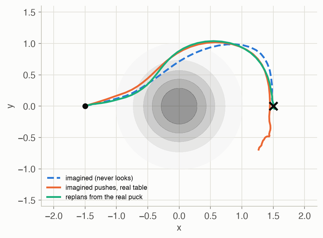
Model predictive control has a built-in defence against compounding errors: every plan starts from the latest real observation, so a planning error lasts at most one step. To see how much that matters, run the same planner twice with the same model. Once it looks at the real puck before every replan. Once it never looks: it replans from the state its own model predicted, so the entire run happens in imagination, and the chosen pushes are then replayed on the real table.
In imagination, every one of the 9 dreamed runs ends within 0.02 of the goal. Replayed on the real table, the same pushes miss by 4.8 on average with the 250-transition models, 0.64 with 1,000 and 0.29 with 4,000. Looking fixes it: with 1,000 or more transitions every run that looks ends within 0.02 of the goal (Figure 3). With 250 transitions even looking fails in some runs (worst miss 2.2): feedback cannot rescue a model that is wrong about which way to go.
The lecture’s world action models use the same idea at scale: DreamZero, when running on the robot, replaces the frames it generated with the real camera frames after each action, so its errors cannot compound ▶ 64:36.
Planners exploit their models
A second danger is subtler. A planner optimizes whatever the model says, and nothing stops it from steering into situations the model never saw, where its predictions are wrong in the planner’s favour. In the toy, the random data only ever pushed with strength up to 1, which is also where the real motor saturates. Let the planner ask for pushes up to 3. The model, never having seen the limit, extrapolates: a push of 3 should be three times as strong. Averaged over 12 plans of 25 steps, allowing stronger pushes improves the imagined cost from 60.1 to 44.4, but the real cost of the same plans only from 61.0 to 58.1 (Figure 9). The planner is mostly fooling itself. Replanning from real observations limits the damage here too: looking at the puck, runs with pushes up to 3 still end within 0.08 of the goal. The Dreamer papers list the same risk for policies trained in imagination: they can exploit world-model errors.
Imagine in a latent space
Most pixels in a camera image do not matter for control, so the next idea is to compress each observation into a small latent vector and do the prediction and the planning there ▶ 25:07. The general recipe: an encoder maps observations to latents, a dynamics model with a recurrent memory predicts the next latent and the reward, and a policy acts on the latent and the memory, so it can be trained purely on imagined rollouts ▶ 25:44.
Ha and Schmidhuber’s World Models (2018) has three separate parts ▶ 27:03: a VAE (vision) that compresses each frame into a latent \(z_t\), whose reconstructions need not be perfect, only informative enough to act on ▶ 28:03; a recurrent network with a mixture-density output (memory), which predicts a distribution over next latents, so several possible futures are not averaged into one ▶ 28:40; and a single linear layer (controller) from latent and memory to action ▶ 29:40. The controller is small on purpose, so that the world model does the representational work, and it is trained by an evolution strategy instead of backpropagation ▶ 30:23. On a car-racing game, removing the memory makes the car leave the track almost at once: a single frame shows position, not speed or the coming curve ▶ 31:42.
Why dreams drift, and the RSSM fix
World Models has a flaw ▶ 33:09. Its memory network is trained on latents encoded from real frames, but in imagination it must feed on its own sampled latents, which come from a slightly different distribution ▶ 33:35. Nothing in training teaches it to produce a good latent from its memory alone. The recurrent state-space model (RSSM) of PlaNet fixes this by splitting the state in two ▶ 34:41: a deterministic memory \(h_t\), which is never sampled and so cannot be corrupted by sampling noise, and a stochastic latent \(z_t\) for what is uncertain. During training, \(z_t\) is inferred from the real observation (the posterior); a prior learns to predict \(z_t\) from \(h_t\) alone, and a KL term keeps the two close, so imagined latents stay where the model was trained ▶ 35:57. In imagination no observation is needed at all: the policy acts, the memory advances, the next latent is drawn from the prior ▶ 36:25.
PlaNet still planned with CEM at every step. Dreamer amortizes that planning into an actor and a critic, trained by backpropagating through imagined rollouts of the frozen model, so at run time the robot simply runs the policy ▶ 38:33. DayDreamer ran the same algorithm on real robots: a quadruped learned to walk from scratch with 1 hour of real interaction ▶ 40:00. Dreamer 3 was the first to collect diamonds in Minecraft from pixels, a task of over 20,000 actions ▶ 42:46. Dreamer 4 does it from offline data only; it pre-trains its dynamics on video without actions and replaces the recurrent memory with a transformer’s key-value cache ▶ 43:40.
Scaling to internet video
The Dreamer latents are compact but specific to one domain: Minecraft, or one robot ▶ 45:26. A model of how the visual world moves in general needs internet-scale video ▶ 46:18, and that runs into token counts first ▶ 46:53. Per-frame patches of a 256 by 256 image give 256 tokens; at 20 frames per second, a 10-second clip has 51,200 ▶ 47:41. But video is extremely redundant ▶ 48:38, and tokenizers compress it along three axes ▶ 48:51: spatially (deeper encoders, fewer tokens per frame), temporally (several frames per token, causally if the model must run in a control loop) ▶ 49:30, and adaptively (more tokens for busy scenes, fewer for static ones) ▶ 50:25. Combined 8 times in each spatial direction and 8 times in time, the 51,200 tokens become 100 ▶ 51:41.
Where do actions go in a model trained mostly on video without actions ▶ 52:18? Three answers (Figure 6):
- Action-conditioned world models (the Dreamer line) take actions as inputs.
- World action models (WAMs) generate future video and actions together as outputs, starting from a pre-trained video model; DreamZero is one ▶ 53:01.
- Video action models (VAMs) keep a pre-trained video model frozen and train only a light inverse dynamics model that reads actions off its features, which needs only robot data for the small part; mimic-video is one ▶ 54:10.
Why use expensive video backbones at all ▶ 55:23? A VLA starts from a vision-language model trained on static images and captions: it knows what “cutting a carrot” means but not how a carrot moves when cut, so robot teleoperation data must teach it the dynamics as well as the control ▶ 56:27. A video model has seen how things move; the robot data then only need to teach control. mimic-video reports 10 times better sample efficiency than VLA architectures (from its abstract). Its oracle experiment: an action decoder given the true future frames succeeds almost always, so the bottleneck is the quality of the predicted video, and better video models should directly give better policies ▶ 59:56.
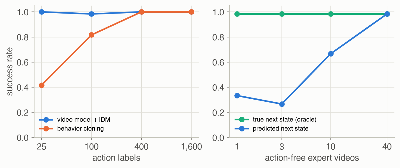
The third toy reproduces both findings. A video model learns from 40 action-free expert videos what the puck does next; an inverse dynamics model learns from \(k\) action-labelled random pushes which push causes a given change. Behavior cloning instead needs \(k\) action-labelled expert transitions. With 25 labels the video model plus decoder succeeds in 100% of runs and behavior cloning in 42%; behavior cloning catches up at 400 labels (Figure 5). Give the decoder the expert’s true next state and it succeeds in about 98% of runs whatever the video model learned; with predicted futures, success goes from 33% with one training video to 98% with 40.
Do we need pixels at all?
Every approach so far decodes back to pixels somewhere. JEPA models do not: they encode the current frame, predict the embedding of the next frame given the action, encode the real next frame with the same encoder, and minimize the distance between the two embeddings, with no decoder and no pixel loss ▶ 68:50. The catch is collapse: an encoder that maps every frame to the same vector makes the prediction error exactly zero, and gradient descent is happy to find it ▶ 69:53. Remedies include a slowly moving (EMA) copy of the encoder for the targets (V-JEPA 2), a frozen pre-trained encoder (DINO-WM), and a regularizer that forces the embeddings to spread out like a Gaussian (the most recent work the lecture cites) ▶ 70:34.
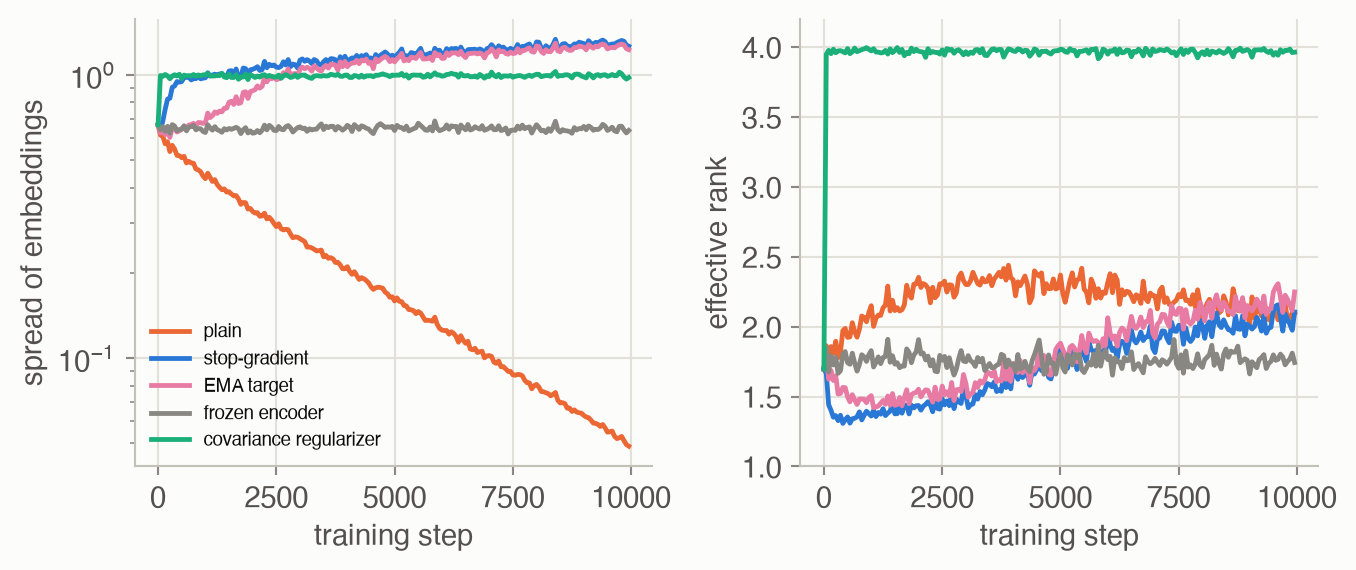
The second toy shows the trap. Observations are a 16-dimensional view of the puck’s state; a linear encoder maps them to 4-dimensional embeddings, and a linear predictor maps (embedding, push) to the next embedding. Trained on prediction error alone, the embeddings shrink from a spread of 0.68 to 0.067 in 10,000 steps, and are still shrinking; this run has the lowest loss of all variants (0.0019), yet a linear readout recovers only 67% of the puck’s position from them. With a regularizer pulling the embeddings’ covariance to the identity, they use all 4 directions (effective rank 3.97) and the readout recovers 99.9% (Figure 7). The other safeguards also prevent collapse here, but leave the embeddings using about two directions.
The lecture closes on its master formula: every family predicts the next state from the current state, an action and a memory, and they differ in how they represent the state, where the actions live, and what data they can use ▶ 71:01.
What to watch for. All three runs use the same world model (1,000 transitions, model 0) and the same planner. The blue dream curves over the upper side of the hill and lands exactly on the goal: by its own model’s account the plan is perfect. The orange puck receives the same pushes on the real table. Its path starts close to the dream’s but runs on a slightly wider arc, so every later push, chosen for where the dream puck was, is a little wrong; it passes the goal and ends below it, 0.7 away, with a few wiggles at the end as the remaining pushes, meant to brake at the goal, act on a puck that is elsewhere. The green puck uses the same model but looks before every replan: its path follows almost the orange course, since the real table behaves the same, but each new plan starts from where the puck really is, and it stops on the goal.
Key concepts & formulae
The lecture writes \(s_t\) for the state, \(a_t\) for the action, \(h_t\) for memory and \(z_t\) for a latent; observations are \(o_t\). The ADM book calls the learned transition model \(T(s' \mid s, a)\) and treats model-based reinforcement learning in its chapter on model-based methods.
What a world model is
\[ \begin{aligned} \text{policy:}\quad & \pi(a_t \mid s_t, g) \\ \text{world model:}\quad & p(s_{t+1} \mid s_t, a_t) \end{aligned} \tag{1}\]
In words. A policy picks what to do for a goal; a world model predicts what will happen if you do it.
Term by term.
- \(g\): the goal, for a VLA a language instruction.
- \(p(s_{t+1} \mid s_t, a_t)\): a distribution, because the same action can have several outcomes. It is the transition model \(P\) of Week 2’s MDP, now learned instead of given.
\[ p(s_{t+1} \mid s_t, a_t, h_t) \tag{2}\]
In words. The next state, predicted from the current state, the action and a memory of the past.
Term by term.
- \(h_t\): memory, needed because the robot’s observation is not the full state (Week 7) and because motion is only visible across frames.
- The action input is what separates a world model from a video model \(p(\text{video} \mid \text{text})\).
Planning with a model
\[ \begin{aligned} a^*_{t:t+H-1} &= \arg\min_{a_{t:t+H-1}} \sum_{k=1}^{H} c(\hat s_{t+k}), \quad \hat s_{t+k} \sim p(\cdot \mid \hat s_{t+k-1}, a_{t+k-1}) \end{aligned} \tag{3}\]
In words. Search for the action sequence whose imagined rollout has the lowest cost, execute its first action, observe, and search again.
Term by term.
- \(\hat s_t = s_t\): each search starts from the latest real state; that reset is what keeps errors from compounding.
- \(c\): the task cost; in the puck toy, the distance to the goal at every step plus the final speed.
- The search here is the cross-entropy method: sample sequences from a Gaussian, keep the best, refit the Gaussian to them, repeat (Week 4 used it over single actions).
\[ e_{k+1} \le L\, e_k + \varepsilon \;\;\Rightarrow\;\; e_H \le \varepsilon\, \frac{L^H - 1}{L - 1} \tag{4}\]
In words. If each predicted step adds a small error \(\varepsilon\), and the dynamics can stretch an existing error by a factor \(L\), the error after \(H\) imagined steps can grow exponentially in \(H\).
Term by term.
- \(e_k\): distance between the imagined and the real state after \(k\) steps.
- \(L\): how much the (model’s) dynamics can amplify a difference in one step; \(L > 1\) for dynamics that spread nearby states apart.
- Why it holds: the next error is the model’s own one-step error plus the old error carried through the dynamics; unroll the recursion and sum the geometric series. With \(L = 1\) the bound is \(\varepsilon H\), linear.
- Numeric check: in the puck toy (1,000 transitions) the error grows 38 times from step 4 to step 40, while the horizon grows 10 times (Figure 2).
Latent world models
\[ \begin{aligned} z_t &= \mathrm{enc}(o_t) \\ p(z_{t+1} \mid a_t, z_t, h_t) &= \textstyle\sum_i \pi_i\, \mathcal{N}(\mu_i, \sigma_i^2) \\ a_t &= W [z_t; h_t] + b \end{aligned} \tag{5}\]
In words. A VAE compresses each frame; a recurrent network predicts a mixture of Gaussians over the next latent; a linear controller acts on latent and memory.
Term by term.
- \(\pi_i, \mu_i, \sigma_i\): weights, means and spreads of the mixture, output by the recurrent network (here \(\pi_i\) is a mixture weight, not a policy).
- \(W, b\): the controller’s only parameters, found by an evolution strategy (CMA-ES) on imagined rollouts.
\[ \begin{aligned} h_t &= f(h_{t-1}, z_{t-1}, a_{t-1}) \\ z_t &\sim q(z_t \mid h_t, o_t) \;\;\text{(training)}, \qquad z_t \sim p(z_t \mid h_t) \;\;\text{(imagination)} \\ \mathcal{L} &= \textstyle\sum_t \big[ -\log p(o_t \mid h_t, z_t) - \log p(r_t \mid h_t, z_t) \\ &\qquad + \mathrm{KL}\big(q(z_t \mid h_t, o_t) \,\|\, p(z_t \mid h_t)\big) \big] \end{aligned} \tag{6}\]
In words. A deterministic memory is updated each step; a stochastic latent is inferred from the observation in training and predicted from memory in imagination; the loss reconstructs observations and rewards and keeps the prior close to the posterior.
Term by term.
- \(f\): a recurrent cell; \(h_t\) is never sampled, so sampling noise cannot corrupt the memory.
- \(q\): the posterior (encoder), which sees the observation; \(p(z_t \mid h_t)\): the prior, which must do without.
- KL term: trains the prior to predict what the posterior would have inferred, so imagined latents stay in the region the decoders understand.
\[ \max_\phi\; \mathbb{E}\Big[\sum_{k=0}^{H-1} \gamma^k \hat r_{t+k} + \gamma^H v_\psi(\hat h_{t+H}, \hat z_{t+H})\Big], \quad \hat a_{t+k} \sim \pi_\phi(\cdot \mid \hat h_{t+k}, \hat z_{t+k}) \tag{7}\]
In words. Roll the actor out inside the frozen world model for \(H\) steps, add up the imagined rewards and the critic’s estimate of what follows, and improve the actor by backpropagating through the model.
Term by term.
- \(\hat r\), \(\hat h\), \(\hat z\): imagined rewards and states; nothing here touches the real environment.
- \(v_\psi\): the critic, trained on the same imagined rollouts; it lets a short horizon \(H\) account for the long-term future.
- Dreamer uses a \(\lambda\)-weighted mix of such returns; the form above shows the idea.
Video and actions
\[ N_{\text{tokens}} = \underbrace{\frac{H W}{p^2}}_{\text{per frame}} \times \underbrace{f\, T}_{\text{frames}} \;\div\; (c_s^2\, c_t) \tag{8}\]
In words. Tokens per frame times the number of frames, divided by the tokenizer’s compression in each spatial direction (\(c_s\), applied twice) and in time (\(c_t\)).
Term by term.
- \(H, W, p\): image height, width and patch size; \(f\): frames per second; \(T\): seconds.
- Numeric check: \(256 \cdot 256 / 16^2 = 256\) tokens per frame, \(\times\, 20 \cdot 10 = 200\) frames, gives 51,200; with \(c_s = c_t = 8\) it becomes 51,200 / 512 = 100.
\[ \begin{aligned} \text{WAM:}\quad & p_\theta(o_{t+1:t+k},\, a_{t:t+k-1} \mid o_{\le t}, \ell) \\ \text{VAM:}\quad & \hat o_{t+1:t+k} \sim p_\theta(\cdot \mid o_{\le t}, \ell), \quad a_{t:t+k-1} = g_\psi(o_t, \hat o_{t+1:t+k}) \end{aligned} \tag{9}\]
In words. A world action model generates the next stretch of video and the actions jointly. A video action model generates (or partially generates) the video plan and lets an inverse dynamics model \(g_\psi\) read off the actions.
Term by term.
- \(\ell\): the language instruction.
- \(g_\psi\): small, trained on robot data only; in the toy, \(k = 1\) and \(g_\psi\) is an MLP of the state and the predicted change.
- Both start from a video model pre-trained on internet video, which supplies the dynamics; mimic-video does not even generate the full video, it uses the model’s features part-way through denoising ▶ 62:10.
Predicting embeddings
\[ \begin{aligned} z_t &= \mathrm{enc}_\theta(o_t), \quad \hat z_{t+1} = \mathrm{pred}(z_t, a_t) \\ \mathcal{L} &= \big\| \hat z_{t+1} - \mathrm{sg}\big[\mathrm{enc}_{\bar\theta}(o_{t+1})\big] \big\|^2 \end{aligned} \tag{10}\]
In words. Predict the embedding of the next observation; compare it with the actual next observation’s embedding, computed by a target encoder that receives no gradient.
Term by term.
- \(\mathrm{sg}\): stop-gradient. \(\bar\theta\): the target encoder’s weights, an EMA of \(\theta\) (V-JEPA 2), or fixed (a frozen encoder).
- Without \(\mathrm{sg}\) and a separate target, \(\mathrm{enc}_\theta \equiv 0\) is a perfect solution: collapse.
- The regularized alternative keeps \(\bar\theta = \theta\) and adds a penalty such as \(\lambda \|\mathrm{Cov}(z) - I\|^2\), which makes the constant solution costly.
- Numeric check: in the toy, stop-gradient alone already prevents collapse (spread 1.28 after 10,000 steps), as does the EMA target (1.26), but only the covariance regularizer uses all 4 directions.
Worked examples
Example 1: the cross-entropy method, iteration by iteration
Planning the first 15 pushes from the start, in the 1,000-transition model: 200 sampled plans per iteration, the 20 cheapest kept.
| iteration | mean cost of samples | best | 20th best | new spread |
|---|---|---|---|---|
| 1 | 46.3 | 41.0 | 43.9 | 0.495 |
| 2 | 43.1 | 39.3 | 41.4 | 0.470 |
| 3 | 41.3 | 39.0 | 39.8 | 0.458 |
| 4 | 40.0 | 37.8 | 39.0 | 0.426 |
| 5 | 39.4 | 38.1 | 38.6 | 0.415 |
| 6 | 39.1 | 37.5 | 38.3 | 0.385 |
The first samples are random pushes. Refitting the Gaussian to the 20 best moves the whole population towards better plans: the mean cost of the samples falls in every iteration, from 46.3 to 39.1. Six iterations do not make the samples agree, though: their spread shrinks only from 0.50 to 0.39. That is enough for MPC, which executes only the first push and then plans again from a warm start. The mean of the last Gaussian is the plan. CEM needs no gradient of the model, which is why it works equally with the true table and with a learned model.
Example 2: compounding, by hand
A model makes a one-step error of \(\varepsilon = 0.01\), and the dynamics stretch any existing error by \(L = 1.1\) per step. After 20 imagined steps the bound of Equation 4 is \(0.01 \times (1.1^{20} - 1)/0.1 = 0.01 \times 57.3 = 0.57\), against \(0.01 \times 20 = 0.2\) if errors simply added up (\(L = 1\)). After 40 steps the two are \(4.4\) and \(0.4\). With replanning from real observations every step, the horizon that matters is 1, and the bound is \(\varepsilon\).
Example 3: the push the planner wanted
The first five pushes of a plan made in the 1,000-transition model with pushes allowed up to 3, and the speed after each push in imagination and on the real table:
| step | push (x, y) | imagined velocity | real velocity |
|---|---|---|---|
| 1 | (+2.15, -0.60) | (+0.33, -0.17) | (+0.19, -0.12) |
| 2 | (+1.67, -0.39) | (+0.60, -0.27) | (+0.38, -0.20) |
| 3 | (+2.01, -0.39) | (+0.88, -0.38) | (+0.56, -0.27) |
| 4 | (+1.88, -0.35) | (+1.10, -0.46) | (+0.73, -0.33) |
| 5 | (+2.18, -0.99) | (+1.28, -0.67) | (+0.87, -0.51) |
The planner asks for pushes well beyond 1, and in imagination the puck accelerates accordingly. On the real table the motor gives no more than 1, so the puck is slower: after five steps its speed is 1.01 instead of the imagined 1.44. Every later step of the plan was chosen for a puck that is not where the plan thinks it is.
Interactive
Dream versus reality, by data size
What to try. At 1,000 transitions the dashed dreams all end on the goal, the orange replays drift off, and the green runs that look end on the goal. Move to 250: the dreams still look perfect (a model always believes itself), but the replays end far away, and even looking does not always help. At 4,000 the replays come closer but still miss.
Asking for more than the motor can give
One 25-step plan from the start, made in the 1,000-transition model (model 0) with pushes limited to the chosen strength. The motor, and the data, stop at 1.
What to try. At 1 the plan respects the motor, and imagination and reality agree closely. Raise the limit: the planner immediately uses the extra strength, the imagined path gets further in 25 steps and its cost drops, but the real puck, held back by the motor, falls behind, and the real cost barely moves. The gap between the two numbers is how much the planner is fooling itself.
Algorithm & code
Planning in a learned model
def rollout(step, s0, actions) -> Array:
    """States s_0..s_H under an action sequence (n, H, 2) from s0 (n, 4)."""
    states = [s0]
    for t in range(actions.shape[1]):
        states.append(step(states[-1], actions[:, t]))
    return np.stack(states, axis=1)                       # (n, H + 1, 4)

def cost(states) -> Array:
    """Distance to the goal at every step, plus the final speed: (n,)."""
    dist = np.linalg.norm(states[:, 1:, :2] - GOAL, axis=-1)
    return dist.sum(axis=1) + 2 * np.linalg.norm(states[:, -1, 2:], axis=-1)

def cem_plan(step, s0, rng, H=15, n=200, elite=20, iters=6, a_max=A_MAX,
             init=None) -> tuple[Array, float]:
    """Cross-entropy method over action sequences in a (true or learned) model.

    Sample n sequences of H pushes from a Gaussian, roll each out in `step`,
    keep the `elite` cheapest, refit the Gaussian, repeat. Returns the final
    mean sequence (H, 2) and its cost according to `step`.
    """
    mu = np.zeros((H, 2)) if init is None else init.copy()
    std = np.full((H, 2), a_max / 2)
    for _ in range(iters):
        A = np.clip(mu + std * rng.standard_normal((n, H, 2)), -a_max, a_max)
        c = cost(rollout(step, np.repeat(s0[None], n, 0), A))
        best = A[np.argsort(c)[:elite]]
        mu, std = best.mean(axis=0), best.std(axis=0) + 0.05
    return mu, float(cost(rollout(step, s0[None], mu[None]))[0])

def run_mpc(plan_step, rng, T=60, H=15, a_max=A_MAX, look=True, start=None):
    """Model predictive control: plan H steps, execute the first push, repeat.

    look=True: every plan starts from the real puck's state. look=False:
    the agent never looks; it replans from the state its own model
    predicted, so the whole run happens in imagination, and the pushes are
    then replayed on the real table. Returns (real path, imagined path),
    each (T + 1, 4); with look=True the two coincide.
    """
    s0 = START_STATE if start is None else start
    real, imag = [s0.copy()], [s0.copy()]
    prev = None
    for _ in range(T):
        here = real[-1] if look else imag[-1]
        # Warm start from the last plan, shifted by one step.
        init = None if prev is None else np.r_[prev[1:], prev[-1:]]
        prev, _ = cem_plan(plan_step, here, rng, H=H, a_max=a_max, init=init)
        a = prev[0]
        real.append(true_step(real[-1], a))
        guess = plan_step(imag[-1][None], a[None])[0]
        imag.append(real[-1] if look else guess)
    return np.array(real), np.array(imag)
import numpy as np
import torch
import torch.nn as nn
from rlc.toys import w08_world as w8
torch.manual_seed(0)
rng = np.random.default_rng(0)
# Data: random transitions of the page's puck table.
s, a, s2 = (torch.tensor(x, dtype=torch.float32)
for x in w8.random_transitions(2000, rng))
scale_in = torch.tensor(w8.IN_SCALE, dtype=torch.float32)
delta = s2 - s
scale_out = delta.std(0)
# World model: (state, push) -> change of state, both scaled to unit size.
model = nn.Sequential(nn.Linear(6, 64), nn.Tanh(), nn.Linear(64, 64),
nn.Tanh(), nn.Linear(64, 4))
opt = torch.optim.Adam(model.parameters(), lr=3e-3)
X = torch.cat([s, a], dim=1) / scale_in
for epoch in range(300):
for idx in torch.randperm(len(X)).split(256):
loss = ((model(X[idx]) - delta[idx] / scale_out) ** 2).mean()
opt.zero_grad(); loss.backward(); opt.step()
@torch.no_grad() # planning needs no gradients of the model
def step(state, push):
x = torch.cat([state, push], dim=-1) / scale_in
return state + model(x) * scale_out
@torch.no_grad()
def cem(state, H=15, n=200, elite=20, iters=6):
"""CEM over push sequences, all n candidates rolled out as one batch."""
goal = torch.tensor(w8.GOAL, dtype=torch.float32)
mu, std = torch.zeros(H, 2), torch.full((H, 2), 0.5)
for _ in range(iters):
A = (mu + std * torch.randn(n, H, 2)).clamp(-1, 1) # (n, H, 2)
x, c = state.expand(n, 4), torch.zeros(n)
for t in range(H):
x = step(x, A[:, t])
c += (x[:, :2] - goal).norm(dim=1)
best = A[c.argsort()[:elite]] # (elite, H, 2)
mu, std = best.mean(0), best.std(0) + 0.05
return mu
# Model predictive control on the real (NumPy) table.
state = torch.tensor(w8.START_STATE, dtype=torch.float32)
for t in range(60):
push = cem(state)[0]
state = torch.tensor(w8.true_step(state.numpy(), push.numpy()),
dtype=torch.float32)
final = (state[:2] - torch.tensor(w8.GOAL, dtype=torch.float32)).norm()
assert final < 0.1, finalThe planner never differentiates the model: CEM only needs to evaluate rollouts, so batching all candidates is the main speed-up. Dreamer replaces this search with an actor trained by backpropagating through the model (Equation 7).
Predicting embeddings, and collapse
def jepa_train(variant, seed, steps=3000, n=512, lr=0.01, tau=0.99,
               lam=1.0) -> dict:
    """Train a linear encoder W and predictor (P_z, P_a) on next-embedding
    error.

    z = o W, prediction = z P_z + a P_a, target z' = o' W_target.
    plain: the target uses W itself and gradients flow into both sides.
    stop-gradient: same W, but the target is treated as a constant.
    EMA target: W_target is a slow moving average of W (no gradient).
    frozen encoder: W stays at its random start; only the predictor learns.
    covariance regularizer: plain, plus lam * ||Cov(z) - I||^2.
    Returns W and the history of the loss, the embeddings' spread and
    their effective rank.
    """
    rng = np.random.default_rng(seed)
    W = rng.standard_normal((OBS_DIM, EMB_DIM)) / np.sqrt(OBS_DIM)
    P_z, P_a = np.eye(EMB_DIM), np.zeros((2, EMB_DIM))
    W_tgt = W.copy()
    hist = {"loss": [], "spread": [], "rank": []}
    for _ in range(steps):
        o, a, o2, _ = jepa_data(n, rng)
        z = o @ W                                      # (n, k)
        target = o2 @ (W if variant in ("plain", "stop-gradient",
                                        "covariance regularizer",
                                        "frozen encoder") else W_tgt)
        r = z @ P_z + a @ P_a - target                 # (n, k) residual
        loss = float((r**2).sum(1).mean())
        dr = 2 * r / n
        dP_z, dP_a = z.T @ dr, a.T @ dr
        dz = dr @ P_z.T                                # through the prediction
        dW = o.T @ dz
        if variant in ("plain", "covariance regularizer"):
            dW -= o2.T @ dr                            # through the target too
        if variant == "covariance regularizer":
            zc = z - z.mean(0)
            C = zc.T @ zc / (n - 1)                    # (k, k)
            loss += lam * float(((C - np.eye(EMB_DIM)) ** 2).sum())
            dW += o.T @ (4 * lam * zc @ (C - np.eye(EMB_DIM)) / (n - 1))
        if variant == "frozen encoder":
            dW = 0 * dW
        W, P_z, P_a = W - lr * dW, P_z - lr * dP_z, P_a - lr * dP_a
        W_tgt = tau * W_tgt + (1 - tau) * W            # used by "EMA target"
        hist["loss"].append(loss)
        hist["spread"].append(float(z.std(0).mean()))
        hist["rank"].append(effective_rank(z))
    return {"W": W, **{k: np.array(v) for k, v in hist.items()}}

def effective_rank(z) -> float:
    """How many directions the embeddings really use: (sum l)^2 / sum l^2
    over the eigenvalues l of their covariance; EMB_DIM if all are equal,
    1 if everything lies on one line."""
    lam = np.clip(np.linalg.eigvalsh(np.cov(z.T)), 0, None)
    return float(lam.sum() ** 2 / (lam**2).sum())
import copy
OBS, EMB = w8.OBS_DIM, w8.EMB_DIM
def train_jepa(target="ema", steps=3000, reg=0.0, tau=0.99):
"""Encoder + predictor on next-embedding error. target: 'same' (gradient
flows into the target too), 'ema' (slow copy, no gradient)."""
torch.manual_seed(0)
enc = nn.Linear(OBS, EMB, bias=False)
pred = nn.Linear(EMB + 2, EMB, bias=False)
enc_tgt = copy.deepcopy(enc).requires_grad_(False)
opt = torch.optim.SGD([*enc.parameters(), *pred.parameters()], lr=0.01)
data_rng = np.random.default_rng(0)
for _ in range(steps):
o, a, o2, _ = (torch.tensor(x, dtype=torch.float32)
for x in w8.jepa_data(512, data_rng))
z = enc(o) # (B, EMB)
z_next = enc(o2) if target == "same" else enc_tgt(o2).detach()
# Squared error summed over the EMB dimensions, averaged over the
# batch (F.mse_loss would also average over dimensions).
err = pred(torch.cat([z, a], dim=1)) - z_next
loss = (err ** 2).sum(dim=1).mean()
if reg:
zc = z - z.mean(0)
cov = zc.T @ zc / (len(z) - 1)
loss = loss + reg * ((cov - torch.eye(EMB)) ** 2).sum()
opt.zero_grad(); loss.backward(); opt.step()
with torch.no_grad(): # EMA update
for p_t, p in zip(enc_tgt.parameters(), enc.parameters()):
p_t.mul_(tau).add_((1 - tau) * p) # in-place ops
return z.std(0).mean().item()
spread_same = train_jepa("same")
spread_reg = train_jepa("same", reg=1.0)
assert spread_same < 0.5 * spread_reg # no safeguard: embeddings shrink
assert abs(spread_reg - 1) < 0.1 # regularized: unit spreaddetach() is the stop-gradient of Equation 10: the target is treated as a constant, so the loss cannot be lowered by moving it. Without it, and without a regularizer, the cheapest way to predict the target is to shrink both towards zero.
Papers
Papers discussed in class
Key papers from the lecture
Guest spotlight
Scott Reed (NVIDIA’s GEAR lab, earlier Google DeepMind, where he led the Gato generalist agent) asked what the right backbone for a robot policy is: the network that encodes cameras, robot state and instructions into a shared representation for predicting actions ▶ 01:09. It decides not only how the policy runs but how much knowledge it can soak up in pre-training and carry to new tasks. The options are training from scratch, starting from a vision-language model (a VLA), and the newer choice of starting from a video model.
On VLAs, he walked from OpenVLA’s binned action tokens ▶ 05:28 to the π models, which pair discrete FAST tokens with a separate flow-matching action expert ▶ 06:15. His reasons: back-propagating flow-matching gradients straight through the language model can destroy its language abilities ▶ 07:13, and a continuous expert never produces the malformed decodes that discrete tokens occasionally do, which on a robot arm is a safety issue ▶ 07:55. He singled out TRI’s large-behavior-model study for its double-blind, statistically careful real-robot evaluation, which found that multi-task pre-training does help ▶ 09:42. The weaknesses he sees: reasoning happens in action space, action outputs are bolted on after pre-training with a risk of forgetting, and data from different robots may stay as separate “data islands” with little transfer between them ▶ 11:35.
World action models predict the world in pixels before or while acting, so pre-training can extract more from each video than action prediction alone ▶ 13:09. DreamZero, of which he is a co-author, encodes frames with a VAE and jointly denoises a chunk of future frames and actions with a block-causal transformer; a “Flash” variant barely denoises the frames and performs as well ▶ 14:01. Its failures mostly came from bad video generation rather than bad action prediction, and performance rose with model size (14B better than 2B), which suggests better video models will directly mean better policies ▶ 20:05. The costs: sampling is expensive, modelling every pixel is probably overkill for control, and context length is limited ▶ 21:20.
From scratch is coming back through human data: wearable sensors and head-mounted cameras can record far more demonstrations than robots can, and recent work shows scaling-law behavior as human data grows ▶ 24:52. He ended “bullish” on world action models combined with large-scale human data ▶ 26:11. In the Q&A he called JEPA-style latent world models promising but unproven, since nobody yet knows which features control needs ▶ 27:02, expected hand-built simulators to keep their place for whole-body control while learned simulators help with contact and deformables, and expected tactile data to be needed in much smaller amounts than video ▶ 30:57.
How it connects to this week. The talk is the lecture’s second half from the inside: the choice between VLMs and video models as the backbone is the choice between “semantics first” and “dynamics first”, and DreamZero’s failure analysis is the same finding as mimic-video’s oracle test and this page’s third toy.
Solved problems
1. Bounding a rollout. A world model has a one-step error of 0.01, and the dynamics stretch errors by at most \(L = 1.1\) per step. Bound the error after 20 imagined steps. How does the bound change if the robot replans from a real observation every 5 steps?
TipSolution
Equation 4 gives \(0.01 \times (1.1^{20} - 1)/0.1 = 0.01 \times 57.3 \approx 0.57\). Replanning from a real observation resets the error to 0 every 5 steps, so the worst error is that of a 5-step rollout: \(0.01 \times (1.1^5 - 1)/0.1 = 0.01 \times 6.1 \approx 0.061\), nine times smaller. That is what looking at the real puck buys in Figure 3.
2. Counting video tokens. A 30-second clip at 30 frames per second, 256 by 256 pixels, 16 by 16 patches. How many tokens per frame and in total without compression? With a tokenizer that compresses 8 times in each spatial direction and 8 times in time?
TipSolution
\(256 \cdot 256 / 16^2 = 256\) tokens per frame and \(30 \cdot 30 = 900\) frames, so 230,400 tokens: far beyond a typical context. With \(c_s = c_t = 8\): \(256/64 = 4\) tokens per frame-group and \(900/8 = 112.5\), about 113 time steps, so about 450 tokens. (Equation 8; temporal compression rounds up at the end of the clip.)
3. Why collapse is a minimum. For the plain JEPA loss \(\|\mathrm{pred}(\mathrm{enc}(o_t), a_t) - \mathrm{enc}(o_{t+1})\|^2\) with linear encoder \(z = oW\) and linear predictor, show that \(W = 0\), \(P_a = 0\) gives zero loss. Why does a stop-gradient target change the picture?
TipSolution
With \(W = 0\) every embedding is 0, the predictor’s output \(0 \cdot P_z + a P_a\) is 0 when \(P_a = 0\), and the target is 0: the loss is exactly 0, its global minimum, while carrying no information about the observation. Gradient descent on both sides moves the target towards the prediction as well as the prediction towards the target, and shrinking everything reduces the loss. With a stop-gradient, the target is a constant at each step; the encoder is then only pushed to make predictions match fixed targets, and shrinking the online embeddings no longer shrinks the target. Whether collapse is then avoided depends on the training dynamics: in this page’s linear toy it is, but the lecture’s methods add an EMA target or a regularizer to make it robust.
4. Which family can use which data? You have (a) internet videos of people cooking, (b) 50 hours of robot play data with actions but no instructions, (c) 5 hours of instruction-labelled teleoperation. Which data can an action-conditioned world model (Dreamer-style), a world action model and a video action model each use, and for what?
TipSolution
An action-conditioned model learns dynamics from (b), including failures, and from (c); (a) has no actions, but Dreamer 4 shows dynamics can be pre-trained on action-free video and then conditioned on actions with a little labelled data. A world action model starts from a video model pre-trained on data like (a), then learns joint video and action prediction from (c); (b) is harder to use because the model is conditioned on instructions, unless the play is relabelled with instructions after the fact. A video action model also starts from (a); its inverse dynamics model can learn from (b) and (c), since it needs (observation, next observation, action) triples, not instructions. This matches the lecture’s comparison of the families ▶ 65:55.
5. Dream or look? Your planner reports that its plan reaches the goal, but the robot misses. Name two different causes, and say which one replanning from real observations fixes.
TipSolution
- Compounding: small one-step errors grow along the imagined rollout, so the plan’s later steps are made for a state the robot is not in. Replanning from real observations fixes this, because every plan starts from the truth and only its first step is executed. (ii) Exploitation: the planner chose actions outside the data, where the model is wrong in its favour, such as pushes beyond the motor’s limit. Replanning limits the damage but does not remove it, since every new plan still trusts the model’s wrong prediction; the fixes are constraining the planner to the data’s range, penalizing model uncertainty, or collecting data where the planner wants to go.
Recap
- A world model predicts consequences of actions. \(p(s_{t+1} \mid s_t, a_t, h_t)\); without the action it is a video model, not a world model. Why it matters: only an action-conditioned model lets a robot ask “what if?”.
- Planning in a model needs feedback. Imagined rollouts compound their errors, and replanning from real observations resets them each step. Why it matters: it is why MPC and closed-loop world action models work while open-loop dreams drift.
- Planners exploit model errors. Optimization finds the actions where the model is wrong in its favour, especially outside the data. Why it matters: every imagination-trained policy inherits the risk.
- Latent world models make imagination cheap. World Models, then RSSM’s deterministic memory and learned prior, then Dreamer’s actor-critic in imagination, up to Dreamer 4’s offline Minecraft diamonds. Why it matters: real-robot learning in hours (DayDreamer) instead of days.
- Video backbones supply dynamics; robot data then teach control. World action models generate video and actions together; video action models decode actions from video features; failures trace back to video quality. Why it matters: it is the main challenger to VLAs as the backbone of generalist policies.
- Predicting embeddings needs a guard against collapse. Stop-gradient targets, EMA or frozen encoders, or covariance regularizers. Why it matters: the lowest prediction loss can be the worst representation.
Cheat sheet & connections
| Name | Formula | Where |
|---|---|---|
| Policy vs world model | \(\pi(a \mid s, g)\) vs \(p(s' \mid s, a)\) | Equation 1 |
| World model ★ | \(p(s_{t+1} \mid s_t, a_t, h_t)\) | Equation 2 |
| MPC | argmin of imagined cost, execute first step, replan | Equation 3 |
| Compounding bound | \(e_H \le \varepsilon (L^H - 1)/(L - 1)\) | Equation 4 |
| World Models (V-M-C) | VAE, MDN-RNN, linear controller | Equation 5 |
| RSSM | \(h_t\) deterministic; \(q(z \mid h, o)\), \(p(z \mid h)\), KL | Equation 6 |
| Dreamer | maximize imagined return + critic | Equation 7 |
| Video tokens | \(\frac{HW}{p^2} f T / (c_s^2 c_t)\) | Equation 8 |
| WAM, VAM | joint \(p(o, a)\); or \(\hat o\) then IDM | Equation 9 |
| JEPA | \(\|\mathrm{pred}(z_t, a_t) - \mathrm{sg}[z_{t+1}]\|^2\) | Equation 10 |
Common pitfalls.
- Calling a text-to-video model a world model: without action conditioning it cannot evaluate your plan.
- Executing a long imagined plan open loop; the dream always looks perfect.
- Letting the planner use actions or states outside the training data, and believing its predicted cost.
- Judging a JEPA by its prediction loss alone; a collapsed encoder has the lowest loss.
- Judging collapse with a scale-invariant probe only: shrinking embeddings still decode well until noise dominates; track their spread and effective rank.
- Comparing world-model families without saying which data each can use.
Connections. Week 2’s transition model \(P(s' \mid s, a)\) is what a world model learns. Week 4 used CEM over actions and Q-learning without a model; Dreamer’s actor-critic is Week 5’s, trained in imagination. Week 3’s compounding errors return here as compounding prediction errors, and the fix is again feedback from the real world. Week 6’s VAEs and flow matching are the encoders and video generators of this week; Week 7’s tokenizers and transformers become video tokenizers and causal video transformers. Week 9 returns to VLAs as generalist policies. In the ADM Companion: learning a model from data, model predictive control and open versus closed loop, which is this page’s “dream or look”.
Resources
- Lecture: video (1:11:48)
- Slides: Official slides (ETH; password-protected) · Community rebuild (unofficial, student repo)
- Guest lecture: Scott Reed (NVIDIA GEAR Lab), What is the right Backbone for Embodied Agents?: video (36:11)
- Papers:
- Learning Universal Policies via Text-Guided Video Generation (Du et al., 2023)
- Training Agents Inside of Scalable World Models (Hafner, Yan & Lillicrap, 2025)
- World Action Models are Zero-shot Policies (Ye et al., 2026)
- Deep Visual Foresight for Planning Robot Motion (Finn & Levine, 2017)
- World Models (Ha & Schmidhuber, 2018)
- Learning Latent Dynamics for Planning from Pixels (Hafner et al., 2019)
- Dream to Control: Learning Behaviors by Latent Imagination (Hafner, Lillicrap, Ba & Norouzi, 2020)
- DayDreamer: World Models for Physical Robot Learning (Wu, Escontrela, Hafner, Abbeel & Goldberg, 2022)
- mimic-video: Video-Action Models for Generalizable Robot Control Beyond VLAs (Pai, Achenbach et al., 2025)